Download
1 / 67
670 likes | 865 Views
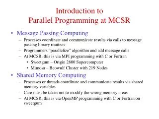
Introduction to Parallel Programming (Message Passing). Francisco Almeida falmeida@ull.es. Parallel Computing Group. Beowulf Computers. Distributed Memory. COTS: Commercial-Off-The-Shelf computers. The Parallel Model. PRAM. Computational Models Programming Models Architectural Models.

E N D
Introduction to Parallel Programming (Message Passing) Francisco Almeida falmeida@ull.es Parallel Computing Group
Beowulf Computers • Distributed Memory • COTS: Commercial-Off-The-Shelf computers
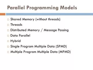
The Parallel Model PRAM • Computational Models • Programming Models • Architectural Models BSP, LogP PVM, MPI, HPF, Threads, OPenMP Parallel Architectures
processor processor processor processor Interconnection Network processor processor processor The Message Passing Model Send(parameters) Recv(parameters)
Network of Workstations Hardware • Distributed Memory • Non Shared Memory Space • Star Topology • Sun Sparc Ultra 1 • 143 Mhz Etherswitch
SGI Origin 2000 Hardware • Shared Dsitributed Memory • Hypercubic Topology • C4-CEPBA • 64 R1000processos • 8 Gb memory • 32 Gflop/s
Digital AlphaServer 8400 Hardware • Shared Memory • BusTopology • C4-CEPBA • 10 Alpha processors21164 • 2 Gb Memory • 8,8 Gflop/s
Drawbacks that arise when solving Problems using Parallelism • Parallel Programming is more complex than sequential. • Results may vary as a consequence of the intrinsic non determinism. • New problems. Deadlocks, starvation... • Is more difficult to debug parallel programs. • Parallel programs are less portable.
MPI CMMD pvm Express Zipcode p4 PARMACS EUI MPI Parallel Libraries Parallel Applications Parallel Languages
MPI • What Is MPI? • Message Passing Interface standard • The first standard and portable message passing library with good performance • "Standard" by consensus of MPI Forum participants from over 40 organizations • Finished and published in May 1994, updated in June 1995 • What does MPI offer? • Standardization - on many levels • Portability - to existing and new systems • Performance - comparable to vendors' proprietary libraries • Richness - extensive functionality, many quality implementations
A Simple MPI Program MPI hello.c #include <stdio.h> #include <string.h> #include "mpi.h" main(int argc, char*argv[]) { int name, p, source, dest, tag = 0; char message[100]; MPI_Status status; MPI_Init(&argc,&argv); MPI_Comm_rank(MPI_COMM_WORLD,&name); MPI_Comm_size(MPI_COMM_WORLD,&p); if (name != 0) { printf("Processor %d of %d\n",name, p); sprintf(message,"greetings from process %d!", name); dest = 0; MPI_Send(message, strlen(message)+1, MPI_CHAR, dest, tag, MPI_COMM_WORLD); } else { printf("processor 0, p = %d ",p); for(source=1; source < p; source++) { MPI_Recv(message,100, MPI_CHAR, source, tag, MPI_COMM_WORLD, &status); printf("%s\n",message); } } MPI_Finalize(); } Processor 2 of 4 Processor 3 of 4 Processor 1 of 4 processor 0, p = 4 greetings from process 1! greetings from process 2! greetings from process 3! mpicc –o hello hello.c mpirun –np 4 hello
. . . 0 1 p One-to-all broadcast Single-node Accumulation One-to-all broadcast M . . . 0 1 p M M M Single-node Accumulation 0 1 Step 1 2 Step 2 . . . Step p p
Second Step 6 7 6 7 2 3 2 3 4 5 4 5 0 1 0 1 First Step 6 7 6 7 2 3 2 3 4 5 4 5 0 1 0 1 Broadcast on Hypercubes
Third Step 6 7 6 7 2 3 2 3 4 5 4 5 0 1 0 1 Broadcast on Hypercubes
MPI Broadcast • int MPI_Bcast( void *buffer; int count; MPI_Datatype datatype; int root; MPI_Comm comm; ); • Broadcasts a message from the process with rank "root" to all other processes of the group
A6 @A7 110 A7 @A6 101 A2 @A3 101 A3 @A2 101 A0 A5@A4 101 A1 A0@A1 000 A1@A0 001 A6 @A7@A4@A5 110 A7 @A6@A5@A4 101 A2 @A3@ A0@A1 101 A3 @A2@ A1@A0 101 A7 @A6@ A5@A4 101 A0@A1 @A2 @A3 000 A1@A0@ A3 @A2 001 Reduction on Hypercubes A6 110 • @ conmutative and associative operator • Ai in processor i • Every processor has to obtain A0@A1@...@AP-1 A7 101 A2 101 A3 101 A5 101 A0 000 A1 001
int MPI_Reduce( void *sendbuf;void *recvbuf;int count;MPI_Datatype datatype;MPI_Op op;int root;MPI_Comm comm;); Reduces values on all processes to a single value processes int MPI_Allreduce( void *sendbuf;void *recvbuf;int count;MPI_Datatype datatype;MPI_Op op;MPI_Comm comm;); Combines values form all processes and distributes the result back to all Reductions with MPI
. . . . . . 0 0 1 1 p p All-To-All BroadcastMultinode Accumulation All-to-all broadcast M1 M2 Mp M0 M0 M0 Single-node Accumulation M1 M1 M1 Mp Mp Mp Reductions, Prefixsums
MPI Collective Operations MPI Operator Operation --------------------------------------------------------------- MPI_MAX maximum MPI_MIN minimum MPI_SUM sum MPI_PROD product MPI_LAND logical and MPI_BAND bitwise and MPI_LOR logical or MPI_BOR bitwise or MPI_LXOR logical exclusive or MPI_BXOR bitwise exclusive or MPI_MAXLOC max value and location MPI_MINLOC min value and location
The Master Slave Paradigm Master Slaves
p= 1 4 dx (1+x2) 0 Computing MPI_Bcast(&n, 1, MPI_INT, 0, MPI_COMM_WORLD); h = 1.0 / (double) n; mypi = 0.0; for (i = myid + 1; i <= n; i += numprocs) { x = h * ((double)i - 0.5); mypi += f(x); } mypi = h * sum; MPI_Reduce(&mypi, &pi, 1, MPI_DOUBLE, MPI_SUM, 0, MPI_COMM_WORLD); 4 2 0.0 0.2 0.4 0.6 0.8 1.0 mpirun –np 3 cpi
void mochila01_sec (void) { unsigned v1; int c, k; for (c = 0; c <= C; c++) f[0][c] = 0; for (k = 1; k <= N; k++) { for (c = 0; c <= C; c++) f[k][c] = f[k-1][c]; if (c >= w[k]) v1 = f[k-1][c - w[k]] + p[k]; if (f[k][c] > v1) f[k][c] = v1; } } The Sequential Algorithm • f[k][c] = max {f[k-1][C], f[k-1][C - W[k] ] + p[k ] for C W[k]} n . . . . . . . . . . . . . . . . C . . . . . . . . . . . . . . . . f[k -] 1] f[k] O(n*C)
Processor k - 1 k Processor . . . . . . . . . . . . . . . . c . . . . . . . . . . . . . . . . f[k-1][c] f[k][c] The Parallel Algorithm 1:void transition (int stage) 2:{ 3: unsigned x; 4: int c, k; 5: k = stage; 6: for (c = 0; c <= C; c++) 7: f[c] = 0; 8: for (c = 0; c <= C; c++) { 9: IN(&x); 10: f[c] = max(f[c], x); 11: OUT(&f[c], 1, sizeof(unsigned)); 12: if (C >= c + w[k]) 13: f[c + w[k]] = x + p[k]; 14: } 15:} f[k][c] = max {f[k-1][C], f[k-1][C - W[k] ] + p[k]}
The Running Time n n -1 + C C
Processor Virtualization n/p Block Mapping C 2 0 1
Processor Virtualization n/p Block Mapping C 2 0 1
Processor Virtualization n/p C 2 0 1
.... (n/p -1)C (p-1)(n/p-1)C The Running Time n/p (n/p -1)C (n/p -1)C C + nC/p = nC 2 0 1
2 0 1 Processor Virtualization n/p C
.... n/p (p-1)(n/p) + nC/p = nC/p 2 0 1 The Running Time n/p n/p n/p C
Block Mapping void transition (void) { unsigned c, k i, inData; for (c = 0; c <= C; c++){ IN(&inData); k = calcInitStage(); for (i = 0; i < width; k++, i++) { f[i] [c] = max(f[i][c], inData); if (c + w[k] <= C) f[i][c + w[k]] = inData + p[k]; inData = f[i][c]; } OUT(&f[i-1][c], 1, sizeof(unsigned)); } } width = N / num_proc; if (f_name < N % num_proc) /* Load Balancing */ width++; int calcInitStage( void ) { return (f_name < N % num_proc) ? f_name * width : (f_name * width) + (N % num_proc) ; }
Cola Cyclic Mapping 2 0 1
Cola 2 0 1 The Running Time (p-1) + n/p C
Cyclic Mapping int bands = num_bands(n); for (i = 0; i < bands; i++) { stage = f_name + i * num_proc; if (stage <= n - 1) transition (stage); } unsigned num_bands (unsigned n) { float aux_f; unsigned aux; aux_f = (float) n / (float) num_proc; aux = (unsigned) aux_f; if (aux_f > aux) return (aux + 1); return (aux); } void transition (int stage) { unsigned x; int c, k; k = stage; for (c = 0; c <= C; c++) f[c] = 0; for (c = 0; c <= C; c++) { IN(&x); f[c] = max(f[c], x); OUT(&f[c], 1, sizeof(unsigned)); if (C >= c + w[k]) f[c + w[k]] = x + p[k]; } }
Advantages and Disadvantages • Block Distribution: • Minimizes the Number of Communications • Penalizes the Startup Time of the Pipeline • Cyclic Distribution: • Minimizes the Startup Time of the Pipeline • May Produce Communications Overhead
Transputer Network - Local Area Network • Transputer Network • Fine Grain • Parallel Communications • Local Area Network • Coarse Grain • Serial Communications
Computational Results Transputers Local Area Network Time Time Processors Processos
The Resource Allocation Problem • M units of an indivisible Resource and a set of N Tasks. • fj(x)Benefit obtained when x unidades of resource are allocated to task j. N max f ( x ) å j j = j 1 N = Subject to x M å j = j 1 £ £ 0 x B , j j = Î xj integer, j 1 , . . . , N ; M , Bj N
RAP- The Sequential Algorithm G[k][m] = max{G[k-1][m-i] + fk(i) / 0 i m } int rap_seq(void) { int i, k, m; for (m = 0; m <= M; n++) G[0][m] = 0; q = a; Q = b; for(k = 0; k < N; k++) { for(m = 0; m <= M; m++) { for (i = 0; i <= m; i++) G[k][m] = max{G[k][m], G[k-1][i] + f[k](m- i)}; } return G[N ][M]; } O(nM2)
Processor k - 1 k Processor . . . . . . . . . . . . . . . . m . . . . . . . . . . . . . . . . G[k-1][m] G[k][m] RAP - The Parallel Algorithm 1:void transition (int stage) 2:{ 3: int m, j, x, k; 4: for( m = 0; m <= M; m++) 5: G[m] = 0; 6: k = stage; 7: for (m = 0; m <= M; m++) { 8: IN(&x); 9: G[m] = max(G[m], x + f(k-1, 0)); 10: OUT(&G[m], 1, sizeof(int)); 11: for (j = m + 1; j <= M; j++) 12: G[j] = max(G[j], x + f(k - 1, j - m)); 13: } /* for m ... */ 14: } /* transition */ G[k][m] = max{G[k-1][m-i] + fk(i) / 0 i m }
The Cray T3E • CRAY T3E • Shared Address Space • Three-Dimensional Toroidal Network
Cola Block - Cyclic Mapping g(p-1) + gM2 n/gp 2 0 1
120 100 10x100 80 100x1000 Time 60 400x1000 45 40 1000x1000 40 35 20 2 30 4 25 0 Time 20 8 2 4 8 16 15 16 Processsors 10 5 0 1 2 5 10 20 40 Grain Computational Results
Linear Model to Predict Communication Performance Time to send N bytes= n + b
PAPI • http://icl.cs.utk.edu/projects/papi/ • PAPI aims to provide the tool designer and application engineer with a consistent interface and methodology for use of the performance counter hardware found in most major microprocessors.
OUT IN Buffering Data Virtual Process nameruns of real processor fname if (name / grain) mod p = fname Processor 1 Processor 0 Processor0 P = 2 Grain = 3 0 1 7 2 3 6 8 ... 4 5 Virtual Processes Size = B SET_BUFIO(1, size)