Download
1 / 9
90 likes | 225 Views
MCP PET Simulation (7) – Pixelated X-tal. 51.0. 0. (not to scale). -51.0. 0. 51.0. X. LSO : Decay time 40ns Lightout : 26,000/MeV 511keV two gammas at the center. 180 deg angle between two gammas. 50mm separation between two modules. Surface: “groundbackpainted”

E N D
MCP PET Simulation (7) – Pixelated X-tal 51.0 0 (not to scale) -51.0 0 51.0 X LSO : Decay time 40ns Lightout : 26,000/MeV 511keV two gammas at the center. 180 deg angle between two gammas. 50mm separation between two modules. Surface: “groundbackpainted” (Unified model) • Dimension : 102x102mm • LSO( 1 pixel => 4x4x25mm3) • pixelated into 24x24(left) • Crystal pitch : 4.25mm • MCP • Photocathode embedded in MCP. • Module = LSOs between 2MCPs.
Single Electron Responses • Pulse Shape • ~500ps rise time(top) • ( real measurement by J-F) • similar value for falling time • assume asymmetric gausian shape • 2. Average gain factor : 10e6 • Single electron gain • ~70% in FWHM. • 3. Transit Time Spread • sigma = 50ps( real measurement by J-F). real measurement cf. Seng’s slides at Picosecond workshop at Lyon08 Simulated pulse shape
Front Side Back Side Readout Scheme • Readout signals from 24 horizontally (vertically) running TLs. • Total 24x2x2 channels for a module. • Position : Anger logic using 5 TLs. • Energy : Sum of two sides( e.g, 5 TL sum w.r.t the maximum for each side) • Timing : Average of maximum Energy TL from each side. TL direction
Number of p.e. ~1447 p.e for 511keV peak. # of p.e.
Energy resolution • 10^6 gain • Sum of 5 TL charge. • 12.0% FWHM • Event around 511keV • ~62% of total events pc
CoincidenceTiming resolution • Select event around 511keV peak • ~38% efficiency( 0.62*0.62) • 10mV threshold LE pickup • 375ps FWHM ns
Reconstructed X coordinate. Position Measurement • Use Anger logic with 5 highest TL’s signal. • Xdet = Sum(Xi*Ei) / Sum(Ei) ( for Vertically running TL in Front) • Ydet = Sum(Yi*Ei)/ Sum(Ei) ( for Horizontally running TL in Back) B C Beam Entering Position(X cor) B : 4.0mm C : 4.5mm Photon( Signal) is highly localized within crystal pitchs( 4.25mm). Position resol. for coincidence event ~ 2mm
Signal Shape at TLs mV ns
Plans • Depth of Interaction(DOI) Simulation. • Position by time difference. • Validation