Download

1 / 28
280 likes | 455 Views
Excel 1. Microsoft Office 2013. Excel Window. 4 Ribbon. 2 File Tab. 1 Title Bar. 3 Top Level Tabs. 5. Group. 7 Name Box. 6 Active Cell. 8 Formula Bar. 9 Column. 10. Row. 11 Sheet Tabs. 12 View Buttons. Excel.

E N D
Excel 1 Microsoft Office 2013
Excel Window 4 Ribbon 2 File Tab 1 Title Bar 3 Top Level Tabs 5. Group 7 Name Box 6 Active Cell 8 Formula Bar 9 Column 10. Row 11 Sheet Tabs 12 View Buttons
Excel • Spreadsheet applications are used to track, analyze, and chart numeric information • Used for business, industry, education, and by individuals who make financial decisions • Microsoft Excel is an electronic spreadsheet program • The term worksheet refers to electronic spreadsheets • A collection of worksheetsis a workbook • There is 1 default sheet in a workbook
Spreadsheets • The function of a spreadsheet allows you to • Compile data • Analyze data • Perform Calculations • Create charts
Words to know: • Vertical information labeled A,B,C – COLUMNS • Horizontal areas labeled 1,2,3 – ROWS • Intersection of a column and row – CELL • The cell with the dark rectangle is called the Active Cell • CELL ADDRESS identifies the coordinates of the intersecting column and row • A1, F10, H233 are examples of cell addresses
Words to know • NAME BOX displays the cell address of the active cell • The ACTIVE CELL and FORMULA BAR displays the data as it is entered • Cells can contain: • Labels (text) • By default, all Labels (text) in cells is left aligned • Values (numbers) • By default, all Values (numbers) in cells are right aligned • Formulas or functions • Dates (serial numbers that can be used included in formuals) • By default, all Dates (serial numbers) in cells are right aligned • RANGE is a selected group of cells • The : indicates a range of cells • B3:D3 is a range of cells • The range of cells include cells B3 through D3
getting around • Left or Right one cell or up and down one row • TAB will move the active cell to the right • SHIFT + TAB will move the active cell to the left • Home takes you to the beginning of a row • Ctrl+Home takes you to A1
Inputting & Changing Data • Key data directly into active cell • F2 or Double Click to make changes in the cell • CLICK INTO THE FORMULA BAR to make changes • Press the DELETE key or just start keying in new data • You DO NOT have to highlight the data in order to delete or change it.
Know your Pointers • Select • Fill • Move
Headers & Footers • Insert Tab > Text Group, Header & Footer button • Header • Left – Name • Center – Insert File Name • Right – Class Period • Footer • Left– Insert Date • Middle-Insert Sheet Name • Right– Teacher’s Name • Always change back to normal view after inserting headers/footers
Be sure to save & Print • Excel files save with an .xlsxfile extension • You can view worksheets in two ways • View in • Regular view – displays the values • Formula view – displays the formulas • Ctrl + ` will toggle you between regular view and formula view (Key above Tab Key) or go to Formulas View Formulas
Useful Ribbons • Alignment • Horizontal • Left Align • Center Align • Right Align • Vertical • Top Align • Middle Align • Bottom Align • Wrap Text • Increase/Decrease Indent • Merge & Center • Orientation • Font • BOLD • Italic • Underline • Increase Font Size • Decrease Font Size • Borders • Fill Color • Font Color • Number • Accounting Number Format • Percent Style • Comma Style • Increase/Decrease Decimal • Cells • Insert and Delete Columns and Rows • Format • Styles • Conditional Formatting • Format as Table • Cell Styles • Editing • AutoSum • Fill • Clear • Sort & Filter • Find & Select To manually wrap text—Alt + Enter
Printing & Page Set-Up Themes • Page Setup • Margins • Orientation • Print Area • Print Titles • Scale to Fit • Automatic Width • Automatic Height • Sheet Options • Print & View Gridlines • Print & View Headings
Inserting Rows & Columns • When you add a row to a spreadsheet, the rows of data below the insertion point are pushed down • When you add a column to a spreadsheet, the columns of data to the right of the insertion point move to the right to make room
Fill Handle • The FillHandle has many uses • It can be used to copy data, copy formulas, and add a series of numbers, days and months • This is AutoFill • The Fill Handle is a small, green dotin the bottom right corner of the active cell
Column Width • To set a column to a specific width, select the column(s) that you want to change • On the Home Tab, in the Cells Group, click Format • Under Cell Size, click Column Width • In the Column width box, type the value you want
Column Width • A column width may have a value of 0 to 255 • This value represents the number of characters that can be displayed in a cell • The default column width is 8.43 characters
AutoFit • If you have text in a cell that extends beyond the default width, select the column • On the Home Tab, in the Cells Group, click Format • Under Cell Size, click AutoFit Column Width • The column will increase in size to the longest text
Row Height • A row height may have a value of 0 to 409 • This value represents a measurement in points • One (1) point equals approximately 1/72 of an inch • The default row height is 15.0 To change row height, go to the Home Tab, cells group, click Format—Click on Row Height—In the box type the value you want
Merge & Center • It is common to center the title, left to right, over the data in the worksheet • The easiest way to do this is to use the Merge and Center option on the Home Tab • Drag through the cells that you want to merge to highlight them • Click on the Merge and Center button, Home Ribbon, to merge the the selected range of cells and to center align the worksheet title
Fill • You can add emphasis to selected cells by changing the Fill color • Click in the active cell, and on the Home Tab, in the Font Group, click the Fill button’s drop down menu • Choose a color from the Fill Color Palette
Borders • By using predefined border styles, you can quickly add a border around a cell or ranges of cells • On the worksheet, select the cell or range of cells you want to add a border to • On the Home Tab, in the Font Group, click the arrow next to Borders and then click a border style
Increase/Decrease Indents • To indent text in a cell, select the cell • On the Home Tab, in the Alignment Group, click repetitively until the text comes to the desired position • For decreasing the indent, select the cell and click the Decrease indent button
Format Painter • Adding formatting to a spreadsheet makes it more attractive and easier for users to find the information they are after • To quickly copy formatting from one part of a sheet to another, use Format Painter
Format Painter • Add all the formatting options you want to at least one cell • Click on that cell to make it active • Click the Format Painter button on the Home Tab, Clipboard Group • Click on the cell that you want to copy the formatting to • If you need to apply the formatting to more than one cell, double-click Format Painter
Sort & Filter • Sorting data helps to quickly visualize and understand data better • To sort, select a column of alphanumeric data in a range of cells • On the Home Tab, in the Sort & Filter Group, do one of the following: • To sort in ascending order, click the A to Z button • To sort in descending order, click the Z to A button
AutoSum • The AutoSum feature is a shortcut to using Excel’s SUM function • It provides a quick way to add up columns or rows in a spreadsheet