Download
1 / 63
630 likes | 762 Views
Missing Data. Michael C. Neale. International Workshop on Methodology for Genetic Studies of Twins and Families Boulder CO 2006 Virginia Institute for Psychiatric and Behavioral Genetics Virginia Commonwealth University Vrije Universiteit Amsterdam. Various forms of missing data.

E N D
Missing Data Michael C. Neale International Workshop on Methodology for Genetic Studies of Twins and Families Boulder CO 2006 Virginia Institute for Psychiatric and Behavioral GeneticsVirginia Commonwealth UniversityVrije Universiteit Amsterdam
Various forms of missing data • Twins volunteer to participate or not • Twins are obtained from hospital records • Attrition during longitudinal studies • Equipment failure: • Systematic (if < value then scored zero) • Random • Structured interviews • Don’t bother asking question 2 if response to Q1 is no • Designs to increase statistical power
Plan of Talk • Review likelihood & Mx facilities • Conceptual view of ascertainment • Ordinal • Continuous • Ascertainment in twin studies • Ordinal • Continuous • Missing data • Systematic (if < value then scored zero) • Random • Structured interviews • Don’t bother asking question 2 if response to Q1 is no
Likelihood approach Advantages & Disadvantages • Usual nice properties of ML remain • Flexible • Simple principle • Consideration of possible outcomes • Re-normalization • May be difficult to compute
Maximum Likelihood Estimates Have nice properties • Asymptotically unbiased • Minimum variance of all asymptotically unbiased estimators • Invariant to transformations • a2 = (a)2 ^ ^
Example: Two Coin Toss 3 outcomes Frequency 2.5 2 1.5 1 0.5 0 HH HT/TH TT Outcome Probability i = freq i / sum (freqs)
Example: Two Coin Toss 2 outcomes Frequency 2.5 2 1.5 1 0.5 0 HH HT/TH TT Outcome Probability i = freq i / sum (freqs)
Non-random ascertainment Example • Probability of observing TT globally • 1 outcome from 4 = 1/4 • Probability of observing TT if HH is not ascertained • 1 outcome from 3 = 1/3 • or 1/4 divided by 'ascertainment correction' of 3/4 = 1/3
Correcting for ascertainment Univariate continuous case; only subjects > t ascertained t N 0.5 0.4 0.3 G 0.2 likelihood 0.1 0 -4 -3 -2 -1 0 1 2 3 4 : xi
Correcting for ascertainment Univariate continuous case; only subjects > t ascertained t N 0.5 0.4 0.3 G 0.2 likelihood 0.1 0 -4 -3 -2 -1 0 1 2 3 4 : xi
Correcting for ascertainment Dividing by the realm of possibilities • Without ascertainment, we compute • With ascertainment, the correction is pdf, N(:ij,Gij), at observed value xi divided by: I-4 N(:ij,Gij) dx = 1 4 t I-4 N(:ij,Gij) dx < 1 Does likelihood increase or decrease after correction?
Ascertainment in PracticeBG Studies • Studies of patients and controls • Patients and relatives • Twin pairs with at least one affected • Single ascertainment pi 6 0 • Complete ascertainment pi = 1 • Incomplete 0 < pi <1 • Linkage studies • Affected sib pairs, DSP etc • Multiple affected families pi = probability that someone is ascertained given that they are affected
Correction depends on model • 1 Correction independent of model parameters: "sample weights" • 2 Correction depends on model parameters: weights vary during optimization • In twin data almost always case 2 • continuous data • binary/ordinal data
High correlation Concordant>t 4 4 Itx ItyN(x,y) dy dx 1 0 ty tx 0 1
Medium correlation 4 4 Itx ItyN(x,y) dy dx 1 0 ty tx 0 1
Low correlation 4 4 Itx ItyN(x,y) dy dx 1 0 ty tx 0 1
Two approaches for twin data in Mx • Contingency table approach • Automatic • Limited to two variable case • Raw data approach • Manual • Multivariate • Moderator / Covariates
Contingency Table Case Binary data • Feed program contingency table as usual • Use -1 for frequency for non-ascertained cells • Correction for ascertainment handled automatically
At least one twin affected tx ty Ascertainment Correction 1-I-4I-4 N(x,y) dy dx + + + + 1 0 + + + + + ty + + + + + + + + + + + + + + + + + + + + + + + + + + tx 0 1
Ascertain iff twin 1 > t 4 4 4 Ity I-4 N(x,y) dx dy Ity N(y) dy = + + + 1 0 + + + + + ty + + + + + + + Twin 1 + + + + + + + + + + + + + + + + + + tx Twin 2 0 1
Contingency Tables • Use -1 for cells not ascertained • Can be used for ordinal case • Need to start thinking about thresholds • Supply estimated population values • Estimate them jointly with model
Mx Syntax Classical Twin Study: Contingency Table ftp://views.vcu.edu/pub/mx/examples/ncbook2/categor.mx G1: Model parameters Data Calc NGroups=4 Begin Matrices; X Lower 1 1 Free Y Lower 1 1 Free Z Lower 1 1 Free W Lower 1 1 End Matrices; ! parameters are fixed by default, unless declared free Begin Algebra; A= X*X'; C= Y*Y'; E= Z*Z'; D= W*W'; End Algebra: End
Mx Syntax Group 2 G2: young female MZ twin pairs Data Ninput=2 CTable 2 2 329 83 95 83 Begin Matrices= Group 1 T full 2 1 Free End Matrices; Covariances A+C+D+E | A+C+D _ A+C+D | A+C+D+E ; Thresholds T ; Options RSidual End
Mx Syntax Group 3 G3: young female DZ twin pairs Data Ninput=2 CTable 2 2 201 94 82 63 Begin Matrices= Group 1 H Full 1 1 Q Full 1 1 T Full 2 1 Free End Matrices; Matrix H .5 Matrix Q .25 Start .6 All Covariances A+C+D+E | H@A+C+Q@D _ H@A+C+Q@D | A+C+D+E / Thresholds T ; Options RSidual NDecimals=4 End
Mx Syntax Group 4 Group 4: constrain variance to 1 Constraint NI=1 Begin Matrices = Group 1 ; I unit 1 1 End Matrices; Constraint I = A+C+E+D ; Option Multiple End Specify 2 t 8 8 Specify 3 t 8 8 End
Raw data approach • Correction not always necessary • ML MCAR/MAR • Prediction of missingness • Correct through weight formula
What can we do with Mx? Normal theory likelihood function for raw data in Mx m ln Li=filn [ 3 wjg(xi,:ij,Gij)] j=1 xi- vector of observed scores onn subjects :ij - vector of predicted means Gij - matrix of predicted covariances - functions of parameters
Likelihood Function Itself The guts of it m • Example: Normal pdf ln Li=fi ln [ 3 wijg(xi,:ij,Gij)] j=1 g(xi,:ij,Gij)- likelihood function
Normal distributionN(:ij,Gij) Likelihood is height of the curve N 0.5 0.4 0.3 G 0.2 likelihood 0.1 0 -4 -3 -2 -1 0 1 2 3 4 : xi
Weighted mixture of models Finite mixture distribution m ln Li=fi ln [ 3 wij g(xi,:ij,Gij)] j=1 j = 1....m models wij Weight for subject i model j e.g., Segregation analysis
Mixture of Normal Distributions Two normals, propotions w1 & w2, different means g 0.5 0.4 w1 x l1 0.3 0.2 w2x l2 0.1 0 xi -4 -3 -2 -1 0 1 2 3 :2 :1 But Likelihood Ratio not Chi-Squared - what is it?
General Likelihood Function Finally the frequencies m • Sample frequencies binary data • Sometimes 'sample weights' • Might also vary over model j ln Li=filn [ 3wj g(xi,:ij,Gij)] j=1 fi- frequency of case i
General Likelihood Function Things that may differ over subjects m • Model for Means can differ • Model for Covariances can differ • Weights can differ • Frequencies can differ ln Li=fi ln [ 3 wij g(xi,:ij,Gij)] j=1 i = 1....n subjects (families)
Raw Ordinal Data Syntax • Read in ordinal file • May use frequency command to save space • Weight uses \mnor function • \mnor(R_M_U_L_K) • R - covariance matrix (p x p) • M - mean vector (1xp) • U - upper threshold (1xp) • L - lower threshold (1xp) • K - indicator for type of integration in each dimension (1xp) • 0: L=-4; 1: U=+4 • 2: Iu; 3: L=-4 U=4 L
Mx Syntax G1: Model parameters Data Calc NGroups=4 Begin Matrices; X Lower 1 1 Free Y Lower 1 1 Free Z Lower 1 1 Free W Lower 1 1 End Matrices; ! parameters are fixed by default, unless declared free Begin Algebra; A= X*X'; C= Y*Y'; E= Z*Z'; D= W*W'; End Algebra: End
Mx Syntax G2: MZ twin pairs Data Ninput=3 Ordinal File=mz.frq Labels T1 T2 Freq Definition Freq ; Begin Matrices= Group 1 T full 2 1 Free F full 1 1 ! Frequency End Matrices; Specify F Freq Covariances A+C+D+E | A+C+D _ A+C+D | A+C+D+E ; Thresholds T ; Frequency F; Options RSidual End
Mx Syntax G3: DZ twin pairs Data Ninput=3 Labels T1 T2 Freq Ordinal File=dz.frq Definition Freq ; Begin Matrices= Group 1 H Full 1 1 Q Full 1 1 T Full 2 1 Free F full 1 1 ! Frequency End Matrices; Specify F Freq Matrix H .5 Matrix Q .25 Start .6 All Covariances A+C+D+E | H@A+C+Q@D _ H@A+C+Q@D | A+C+D+E / Thresholds T ; Frequency F ; Options RSidual NDecimals=4 End
Mx Syntax Group 4: constrain variance to 1 Constraint NI=1 Begin Matrices = Group 1 ; I unit 1 1 End Matrices; Constraint I = A+C+E+D ; Option Multiple End Specify 2 t 8 9 Specify 3 t 8 9 End
Ascertainment additional commands Begin Algebra; M=(A+C+E|A+C_A+C|A+C+E); N=(A+C+E|h@A+C_h@A+C|A+C+E); J=I-\mnor(M_Z_T_T_Z); ! Z = [0 0] K=I-\mnor(N_Z_T_T_Z); ! DZ case End Algebra; Weight J~; ! for MZ group Weight K~; ! DZ group Why inverse of J and K?
Correcting for ascertainment Linkage studies • Multivariate selection: multiple integrals • double integral for ASP • four double integrals for EDAC • Use (or extend) weight formula • Precompute in a calculation group • unless they vary by subject
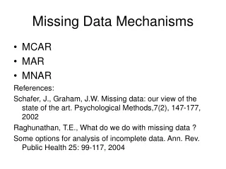
When ascertainment is NOT necessary Little & Rubin Terminology • Various flavors of missing data mechanisms • MCAR: Missing completely at random • MAR: Missing at random • NMAR: Not missing at random
Simulation: 3 types of missing data • Selrand: MCAR • missingness function of independent random variable • Selonx: MAR • missingness predicted by other measured variable in analysis + MCAR • Selony: NMAR • missingness mechanism related to ''residual" variance in dependent variable
Method • Simulate bivariate normal data X,Y • Sigma = 1 .5 • .5 1 • Mu = 0, 0 • Make some variables missing • Generate independent random normal variable, Z, if Z>0 then Y missing • If X>0 then Y missing • If Y>0 then Y missing • Estimate elements of Sigma & Mu • Constrain elements to population values 1,.5, 0 etc • Compare fit • Ideally, repeat multiple times and see if expected 'null' distribution emerges
Method • Check to see if estimates ‘look right’ • Quantify ‘look right’ • Test model with parameters fixed to population values • Look at chi-squared • Repeat! • Examine distribution of chi-squareds
R simulation script: selrand.R r<-0.5 #Correlation (r) N<-1000 #Number of pairs of scores outfile<-"selrand.rec" #output file for the simulation vals<-matrix(rnorm((N*3)),,3); #3 random normals per pair of observed scores rootr<-sqrt(r); #Square root of r root1mr<-sqrt(1-r); #Square root of (1-r) #Data generation follows: pairs<-matrix(cbind(rootr*vals[,1]+root1mr*vals[,2],rootr*vals[,1] +root1mr*vals[,3]),,2) # pairs now contains pairs of scores drawn from population # with unit variances and correlation r
R simulation script: selrand.R # Now to make some of the scores missing, using a loop for (i in 1:N) { x<-rnorm(1,0,1) # x is an independent random number from N(0,1) if (x>0) pairs[i,2] <- NA } write.table (pairs,file=outfile,row.names=FALSE,na=".",col.names=FALSE)
R simulation script: selonx.R # Now to make some of the scores missing, using a loop for (i in 1:N) { if (pairs[i,1]>0) pairs[i,2] <- NA } write.table(pairs,file=outfile,row.names=FALSE,na=".", col.names=FALSE) # note how missingness of 2nd column of pairs depends on # value of 1st column
R simulation script: selony.R # Now to make some of the scores missing, using a loop for (i in 1:N) { if (pairs[i,2]>0) pairs[i,2] <- NA } write.table(pairs,file=outfile,row.names=FALSE,na=".", col.names=FALSE) # note how missingness of 2nd column of pairs depends on # value of 2nd column itself
Mx Script Rather basic, like Monday morning Estimate pop cov matrix of X&Y, with Y observed iff X>0 Data ngroups=1 ninput=2 Rectangular file=selonx.rec Begin Matrices; a sy 2 2 free ! covariance of x,y m fu 1 2 free ! mean of x,y End Matrices; Means M / Covariance A / matrix a 1 .3 1 bound .1 2 a 1 1 a 2 2 option rs mu issat end fix all matrix 1 a 1 .5 1 matrix 1 m 0 0 end