Download
1 / 21
380 likes | 1.15k Views
Dispersion of Air Pollutants. The dispersion of air pollutants is primarily determined by atmospheric conditions. If conditions are superadiabatic a great deal of vertical air movement will result and dispersion is enhanced.

E N D
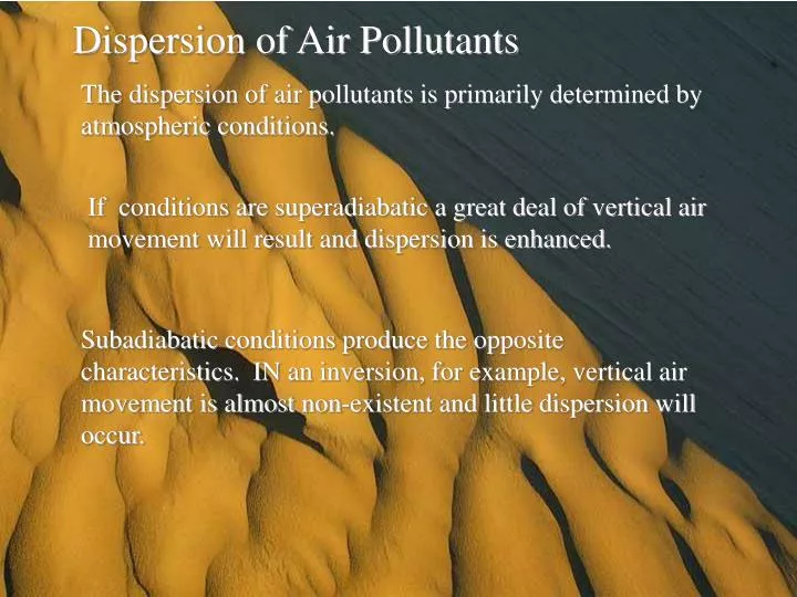
Dispersion of Air Pollutants The dispersion of air pollutants is primarily determined by atmospheric conditions. If conditions are superadiabatic a great deal of vertical air movement will result and dispersion is enhanced. Subadiabatic conditions produce the opposite characteristics. IN an inversion, for example, vertical air movement is almost non-existent and little dispersion will occur.
)h = plume rise above stack, m u = average wind speed, m/sec )T/)z = prevailing lapse rate, oC/m Vs = stack gas exit velocity, m/s d = stack diameter, m Ta = temperature of atmosphere, oC Ts = temperature of stack gas, oC F = buoyancy flux, m4sec-3 )h = 2.6 [F/( u S)]1/3 Plume Rise As you can see from the preceding figure the height a plume rises is very important. No theoretical model has been developed to predict plume rise, but several good empirical models have been developed. One of those is presented below: F = [gVsd2(Ts – Ta)] / [4 (Ta + 273)] S = [g/(Ta + 273)] [ ()T/)z) + 0.01]
)h = 2.6 [F/( u S)]1/3 Example A stack has an emission exiting at 3 m/sec through a stack with a diameter of 2 m. The average wind speed is 6 m/sec. The air temperature at the stack exit elevation is 28oC and the temperature of the emission is 167oC. The atmosphere is at neutral stability. What is the expected rise of the plume? At neutral stability, )T/)z = 0.01 oC/m F = [9.8 x 3 x 22 x (167 – 28)] / [ 4 (28 + 273)] = 13.6 S = [9.8 / (28 + 273)] ( 0.01 + 0.01) = 6.51 x 10⁻⁴ )h = 2.6 [13.6 / ( 6 x 6.51 x 10-4)]1/3 = 40 m
Dispersion Modeling C(x,y,z) = [Q/(2 B u Fy Fz)] exp[ -1/2 [(y / Fy)2 + (z / Fz)2]] Dispersion is the process of spreading out the emission over a large area thereby reducing the concentration of the pollutants. Plume dispersion is in two dimensions: horizontal and vertical. It is assumed that the greatest concentration of the pollutants is on the plume centerline in the direction of the prevailing wind. The further the away from the centerline the lower the concentration. The spread of the plume is approximated by Gaussian probability curve C(x, y, z) = concentration at some point in coordinate space, kg,m3 Q = source strength, kg/sec Fy,Fz= standard deviation of the dispersion in the y and z directions y = distance crosswind horizontally, m z = distance crosswind vertically, m z is in the vertical direction, y is in the horizontal crosswind direction, and x is the downwind direction
C(x,y,z) = [Q/(2 B u Fy Fz)] exp[ -1/2 [(y / Fy)2 + (z / Fz)2]] The degree of dispersion is controlled by the standard deviations in the equation. When F is large the spread is great, so the concentration is low (the mass is spread out over a larger area.) Dispersion is dependent on both atmospheric stability and distance from the source The values for the standard deviations for this equation can be found using tables which have been prepared for that purpose. To use the table you first must estimate the atmospheric stability
C(x,y,z) = [Q/(2 B u Fy Fz)] exp[ -1/2 [(y / Fy)2 + (z - H / Fz)2]] Consider this figure: A plume emitted from a stack has an effective height H (you have to calculate )h). The centerline of the plume, z, is then H and the dispersion equation becomes: This equation and the one presented previously hold as long as the ground does not influence the diffusion (the plume hits the ground)
C(x,y,z) = [Q/(2 B u Fy Fz)] exp[ -1/2 (y / Fy)2] x {exp[-1/2[(z + H) / Fz)2] + exp [ -1/2 [(z – H)/Fz]]2} Since most pollutants are not absorbed by the ground, and they can not diffuse into the ground the equations above will not work when there is influence from the ground. One way of accounting for this influence is to assume all pollutants are reflected by the ground. A new equation can be written based on this assumption:
Example A source emits 0.01 kg/sec of a Sox on a sunny summer afternoon with an average wind speed of 4 m/sec. The effective stack height has been determined to be 20 m. Find the ground level concentration 200 m downwind from the stack. A sunny afternoon would give curve B
Now from the figures: Fy = 36 m Fz = 20 m
C(x,y,z) = [Q/(2 B u Fy Fz)] exp[ -1/2 (y / Fy)2] x {exp[-1/2[(z + H) / Fz)2] + exp [ -1/2 [(z – H)/Fz]]2} Now x = 200 m, y = 0, z = 0 m, and: C(200,0,0) = [0.01 / (2 x 3.14 x 4 x 36 x 20)] x { exp[ –1/2(0/36)] x {exp[ -1/2 x [(0 – 20)/20]2] = exp[ -1/2 x [(0 + 20)/20]2]}} = 6.7 x 10⁻⁷ kg/m3 = 670 :g/m3
C(x,y,z) = [Q/(2 B u Fy Fz)] exp[ -1/2 (y / Fy)2 ] C(x,y,z) = [Q/(2 B u Fy Fz)] Special Conditions If the measurement is taken at ground level and the plume is emitted at ground level (Z = 0, H = 0): If the emission is at ground level and the pollutant is measured at ground level on the center line in the direction of the wind (H = 0, z = 0, and y = 0), the equation is even further simplified to:
Control of Pollution from Automobiles Important points requiring control: Evaporation loss from fuel tank Evaporation of HC’s from carburetor Emission of unburned gas and partially oxidized HC’s from crankcase NOx., HC’s, and CO in the exhaust
Control of the potential emission points Evaporation form the gas tank can be eliminated by use of gas tank caps that prevent vapor escaping Losses from carburetors can be reduced by using activated carbon canisters that adsorb vapors emitted when the engine is turned off and hot gasoline in the carburetor vaporizes. The vapors are purged from the canister by air when the car is restarted and burned in the engine Crankcase emissions have been eliminated by recycling crankcase gases into the intake manifold and the installation of the positive crankcase ventilation valve (PCV).
Exhaust Emissions 60% of the HC’s and almost all of the NOx, CO, and lead come from the exhaust. The quantity of emissions changes with the operating conditions of the vehicle.
When the car is accelerating the combustion is efficient (low CO and HC), but high amounts of NOx are produced. When the car is decelerating there are low amounts of NOx produced but high amounts of HC’s due to partially burned fuel. This makes it difficult to determine how much pollution a particular engine design produces. The EPA has developed a standard test to make this determination. The test includes a cold start, cruising with a simulated load, and a hot start.
Exhaust emission control techniques Tuning the engine to burn fuel efficiently Installation of catalytic reactors Engine modifications
Engine Tuning A well tuned engine is the first line of defense for controlling automobile emissions
Catalytic Converters Oxidize CO and HC’s to CO2 and H2O Most common catalyst - platinum Problems: Fouled by some gasoline additives like lead (this is why lead has been eliminated from gasoline) Sulfur in gasoline converted to particulate SO3
Redesign of internal combustion engines Cylinder configuration Fuel injectors