Download
1 / 111
1.11k likes | 1.3k Views
Review of Top 10 Concepts in Statistics (reordered slightly for review the interactive session). NOTE: This Power Point file is not an introduction, but rather a checklist of topics to review. Top Ten #10. Qualitative vs. Quantitative. Qualitative. Categorical data: success vs. failure

E N D
Review of Top 10 Conceptsin Statistics(reordered slightly for review the interactive session) NOTE: This Power Point file is not an introduction, but rather a checklist of topics to review
Top Ten #10 • Qualitative vs. Quantitative
Qualitative • Categorical data: success vs. failure ethnicity marital status color zip code 4 star hotel in tour guide
Qualitative • If you need an “average”, do not calculate the mean • However, you can compute the mode (“average” person is married, buys a blue car made in America)
Quantitative • Two cases • Case 1: discrete • Case 2: continuous
Discrete (1) integer values (0,1,2,…) (2) example: binomial (3) finite number of possible values (4) counting (5) number of brothers (6) number of cars arriving at gas station
Continuous • Real numbers, such as decimal values ($22.22) • Examples: Z, t • Infinite number of possible values • Measurement • Miles per gallon, distance, duration of time
Graphical Tools • Pie chart or bar chart: qualitative • Joint frequency table: qualitative (relate marital status vs zip code) • Scatter diagram: quantitative (distance from CSUN vs duration of time to reach CSUN)
Hypothesis TestingConfidence Intervals • Quantitative: Mean • Qualitative: Proportion
Top Ten #9 • Population vs. Sample
Population • Collection of all items (all light bulbs made at factory) • Parameter: measure of population (1) population mean (average number of hours in life of all bulbs) (2) population proportion (% of all bulbs that are defective)
Sample • Part of population (bulbs tested by inspector) • Statistic: measure of sample = estimate of parameter (1) sample mean (average number of hours in life of bulbs tested by inspector) (2) sample proportion (% of bulbs in sample that are defective)
Top Ten #1 • Descriptive Statistics
Measures of Central Location • Mean • Median • Mode
Mean • Population mean =µ= Σx/N = (5+1+6)/3 = 12/3 = 4 • Algebra: Σx = N*µ = 3*4 =12 • Sample mean = x-bar = Σx/n • Example: the number of hours spent on the Internet: 4, 8, and 9 x-bar = (4+8+9)/3 = 7 hours • Do NOT use if the number of observations is small or with extreme values • Ex: Do NOT use if 3 houses were sold this week, and one was a mansion
Median • Median = middle value • Example: 5,1,6 • Step 1: Sort data: 1,5,6 • Step 2: Middle value = 5 • When there is an even number of observation, median is computed by averaging the two observations in the middle. • OK even if there are extreme values • Home sales: 100K,200K,900K, so mean =400K, but median = 200K
Mode • Mode: most frequent value • Ex: female, male, female • Mode = female • Ex: 1,1,2,3,5,8 • Mode = 1 • It may not be a very good measure, see the following example
Measures of Central Location - Example Sample: 0, 0, 5, 7, 8, 9, 12, 14, 22, 23 • Sample Mean = x-bar = Σx/n = 100/10 = 10 • Median = (8+9)/2 = 8.5 • Mode = 0
Relationship • Case 1: if probability distribution symmetric (ex. bell-shaped, normal distribution), • Mean = Median = Mode • Case 2: if distribution positively skewed to right (ex. incomes of employers in large firm: a large number of relatively low-paid workers and a small number of high-paid executives), • Mode < Median < Mean
Relationship – cont’d • Case 3: if distribution negatively skewed to left (ex. The time taken by students to write exams: few students hand their exams early and majority of students turn in their exam at the end of exam), • Mean < Median < Mode
Dispersion – Measures of Variability • How much spread of data • How much uncertainty • Measures • Range • Variance • Standard deviation
Range • Range = Max-Min > 0 • But range affected by unusual values • Ex: Santa Monica has a high of 105 degrees and a low of 30 once a century, but range would be 105-30 = 75
Standard Deviation (SD) • Better than range because all data used • Population SD = Square root of variance =sigma =σ • SD > 0
Empirical Rule • Applies to mound or bell-shaped curves Ex: normal distribution • 68% of data within + one SD of mean • 95% of data within + two SD of mean • 99.7% of data within + three SD of mean
Standard Deviation Total variation = 34 • Sample variance = 34/4 = 8.5 • Sample standard deviation = square root of 8.5 = 2.9
Measures of Variability - Example The hourly wages earned by a sample of five students are: $7, $5, $11, $8, and $6 Range: 11 – 5 = 6 Variance: Standard deviation:
Graphical Tools • Line chart: trend over time • Scatter diagram: relationship between two variables • Bar chart: frequency for each category • Histogram: frequency for each class of measured data (graph of frequency distr.) • Box plot: graphical display based on quartiles, which divide data into 4 parts
Top Ten #8 • Variation Creates Uncertainty
No Variation • Certainty, exact prediction • Standard deviation = 0 • Variance = 0 • All data exactly same • Example: all workers in minimum wage job
High Variation • Uncertainty, unpredictable • High standard deviation • Ex #1: Workers in downtown L.A. have variation between CEOs and garment workers • Ex #2: New York temperatures in spring range from below freezing to very hot
Comparing Standard Deviations • Temperature Example • Beach city: small standard deviation (single temperature reading close to mean) • High Desert city: High standard deviation (hot days, cool nights in spring)
Standard Error of the Mean Standard deviation of sample mean = standard deviation/square root of n Ex: standard deviation = 10, n =4, so standard error of the mean = 10/2= 5 Note that 5<10, so standard error < standard deviation. As n increases, standard error decreases.
Sampling Distribution • Expected value of sample mean = population mean, but an individual sample mean could be smaller or larger than the population mean • Population mean is a constant parameter, but sample mean is a random variable • Sampling distribution is distribution of sample means
Example • Mean age of all students in the building is population mean • Each classroom has a sample mean • Distribution of sample means from all classrooms is sampling distribution
Central Limit Theorem (CLT) • If population standard deviation is known, sampling distribution of sample means is normal if n > 30 • CLT applies even if original population is skewed
Top Ten #5 • Expected Value
Expected Value • Expected Value = E(x) = ΣxP(x) = x1P(x1) + x2P(x2) +… Expected value is a weighted average, also a long-run average
Example • Find the expected age at high school graduation if 11 were 17 years old, 80 were 18 years old, and 5 were 19 years old • Step 1: 11+80+5=96
Top Ten #4 • Linear Regression
Linear Regression • Regression equation: • =dependent variable=predicted value • x= independent variable • b0=y-intercept =predicted value of y if x=0 • b1=slope=regression coefficient =change in y per unit change in x
Slope vs Correlation • Positive slope (b1>0): positive correlation between x and y (y increase if x increase) • Negative slope (b1<0): negative correlation (y decrease if x increase) • Zero slope (b1=0): no correlation(predicted value for y is mean of y), no linear relationship between x and y
Simple Linear Regression • Simple: one independent variable, one dependent variable • Linear: graph of regression equation is straight line
Example • y = salary (female manager, in thousands of dollars) • x = number of children • n = number of observations
Slope (b1) = -6.5 • Method of Least Squares formulas not on BUS 302 exam • b1= -6.5 given Interpretation: If one female manager has 1 more child than another, salary is $6,500 lower; that is, salary of female managers is expected to decrease by -6.5 (in thousand of dollars) per child
Intercept (b0) • b0 = 44.33 – (-6.5)(2.33) = 59.5 • If number of children is zero, expected salary is $59,500