Download
1 / 19
190 likes | 364 Views
GLACIAL ISOSTATIC ADJUSTMENT AND COASTLINE MODELLING. Glenn Milne Dept of Geological Sciences University of Durham, UK. Outline. General GIA • What is GIA? • Key observables • General model components • Constraining model parameters (2) Modelling coastline evolution

E N D
GLACIAL ISOSTATIC ADJUSTMENT AND COASTLINE MODELLING Glenn Milne Dept of Geological Sciences University of Durham, UK
Outline • General GIA • • What is GIA? • • Key observables • • General model components • • Constraining model parameters • (2) Modelling coastline evolution • • General idea • • Predicting GIA-induced sea-level change • • Example predictions
Oxygen Isotope Record 18O/16O(sample) - 18O/16O(standard) d18O=1000 x 18O/16O(standard)
GLACIAL ISOSTATIC ADJUSTMENT Surface Mass Redistribution Earth Earth Response • Relative sea level • Geopotential • Rotation vector • 3D solid surface deformation Model Surface load + Rotational potential Rheological Earth model Constraints on surface mass redistribution Better understanding of GIA process Constraints on Earth rheology
GIA MODEL Earth Forcing Earth Rheology Impulse response formalism Linear Maxwell rheology 1D structure Rotational potential Surface loading Euler equations Ice Other? Interdisciplinary approach Ice dammed lakes Sediment redistribution Ocean Sea-level equation Ice history and earth rheology are the key inputs
Constraining Model Parameters • Largest uncertainties associated with ice sheet histories and earth rheology • Near-field data give best constraints on local ice histories • Near-field and far-field data can be effectively used to constrain earth viscosity structure • Far-field sea-level data give best constraints on integrated ice melt signal • Both forward and inverse modelling techniques are used
Modelling Coastline Evolution (Associated with GIA) • Position of coastline is influenced by rising/falling relative sea level AND advancing or retreating marine-based ice
Modelling Coastline Evolution Driven by GIA-Induced Sea-Level Changes • Choose optimal model parameters and predict changes in relative sea level for period of interest • Compute palaeotopography via the relation • Accuracy of prediction will depend on accuracy of the present-day topography data set and the accuracy of the relative sea-level prediction • GIA model does not include tectonic motions or sediment flux (associated with marine or fluvial processes)
Eustatic Sea-Level Change • Mass conservation • Earth is rigid and non-rotating • Ice and water have no mass
Glaciation-Induced Sea-Level Change S(q,f,t) = G(q,f,t) – R(q,f,t) + HG(t) • Geoid perturbation,G(q,f,t) • geopotential perturbed directly by surface mass redistribution and changing rotational potential and indirectly by earth deformation caused by these forcings • Solid surface perturbation, R(q,f,t) • vertical earth deformation associated withsurface mass redistribution and changing rotational potential • Surface mass conservation, HG(t) • VOW(t) = G(q,f,t) – R(q,f,t) +HG(t)AO • HG(t) = VOW(t) AO-1 – AO-1 G(q,f,t) – R(q,f,t) • “eustatic” “syphoning”
Sea-Level Model ●Original theory published by Farrell and Clark (1976). ●Theory extended to include: (1) Time-dependent shorelines (Johnston 1993; Peltier 1994; Milne et al. 1999). (2) Glaciation-induced perturbations to Earth rotation (Han and Wahr 1989; Bills and James 1996; Milne and Mitrovica 1996; 1998). (3) The influence of marine-based ice sheets (Milne 1998; Peltier 1998).
Some Comments on the Sea-Level Algorithm • Computing ∆G and ∆R requires knowledge of the sea-level change since this is a key component of surface load. Iterative process required at each time step in computation. • Sea loading in given by C(θ,Φ,t) S(θ,Φ,t). Continent function can only be determined when RSL is known. Iterative process required over each glacial cycle. • High spatial resolution computations are computationally intensive (CPU and disk space).
20 kyr BP 10 kyr BP