CS 2262: Numerical Methods

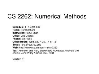
1. CS 2262: Numerical Methods Schedule: TTh 3:10-4:30 Room: Turead 0229 Instructor: Rahul Shah Office: 285 Coates Phone: 578-4355 Office Hours: Wed 2:30-4:30, Th 11-12 Email: rahul@csc.lsu.edu Web: http://www.csc.lsu.edu/~rahul/2262 Text: Atkinson and Han, Elementary Numerical Analysis, 3rd edition, John Wiley & Sons, Inc., 2004 Grader: ?

2. Grading • Midterm : 30 % • Final : 30% • Homework/Project: 25+10 = 35% • Class Participation : 5% • Relative – on the curve • Homeworks will involve writing Matlab programs …about 4 to 5 of them • Mini project will involve solving real-life problem using Matlab and/or C

3. Prerequisites and Background • Math 1552 and • CS 1251 or 1351 or 2290 • The course will involve concepts from • Calculus • Linear Algebra • Programming • Matlab • C

4. Applications of this course Sales data Search Engines Network problems Data Mining Fluid dynamics Algorithms/Optimization Numerical Methods Stock Market Solving large scale systems

5. Course Contents • Foundations: Calculus, Computer Architecture, Matlab • Taylor Series • Root Finding • Polynomial Interpolation • Numerical Integration/Differentiation • Linear Equations/Matrices • Differential Equations

6. Overview • Taylor Series • Evaluationg functions like sin x, ex etc • Processors only have support for additions and multiplications • Errors involved, number of iterations needed

7. Overview: Root finding • Reverse process of evaluating the function • Given function f, find the value of x such that f(x) = 0 • Methods for general functions • Methods for polynomials • Rate of convergence

8. Interpolation • Given a set of points (x1, y1) , (x2, y2), …, (xn, yn) • Find a polynomial which passes through them • Find a line which fits these the best • Find a smooth curve which passes through them

9. Matrices • Given a set of n linear equations in variables x1, x2, x3, …, xn • Find the values of xi s • Find best values of xi s • Linear programming , Optimization • Find Eigenvalues of the matrix • Google • Differential Equations

10. Differential Equations • Modelling/Simulations of Engineering systems • Population Modeling • Financial Models, Stocks/Options pricing

11. Motivation1: Modelling • Traditionally, engineering and science had a two-sided approach to understanding a subject: the theoretical and the experimental. More recently, a third approach has become equally important: the computational. • Traditionally we would build an understanding by building theoretical mathematical models, and we would solve these for special cases. For example, we would study the flow of an incompressible irrotational fluid past a sphere, obtaining some idea of the nature of fluid flow. But more practical situations could seldom be handled by direct means, because the needed equations were too difficult to solve. Thus we also used the experimental approach to obtain better information about the flow of practical fluids. The theory would suggest ideas to be tried in the laboratory, and the experiemental results would often suggest directions for a further development of theory.

12. Modeling contd Theoretical Science Computational Science Experimental Science

13. Modeling: Population • This is the simplest model for population growth. Let N(t) denote the number of individuals in a population (rabbits, people, bacteria, etc). Then we model its growth by • N’(t) = cN(t), t≥ 0, N(t0) = N0 • The constant c is the growth constant, and it usually must be determined empirically. • Over short periods of time, this is often an accurate model for population growth. For example, it accurately models the growth of US population over the period of 1790 to 1860, with c = 0.2975.

14. Population Data

15. Predator-Prey • Let F(t) denote the number of foxes at time t; and let R(t) denote the number of rabbits at time t. A simple model for these populations is called the Lotka-Volterra predator-prey model: • dR/dt = a [1 − bF(t)] R(t) • dF/dt = c [−1 + gR(t)] F(t) • with a, b, c, g positive constants. • If one looks carefully at this, then one can see how it is built from the logistic equation. In some cases, this is a very useful model and agrees with physical experiments. Of course, we can substitute other interpretations, replacing foxes and rabbits with other predator and prey. The model will fail, however, when there are other populations that affect the first two populations in a significant way.

16. Motivation2: Google • Term frequency, location, meaning based search engines : Altavista, Lycos etc • Spamming • Google used social concepts to reduce effect of spamming • A webpage is good if many good webpages link to it • So how to find goodness score

17. Google contd.. • Say there a n webpages • Construct a n x n probability matrix • With A[i,j] = likelihood that a user will jump to page j from i • Find dominant eigenvalue of this matrix • Corresponding eigenvector gives the goodness scores • How to solve the problem on such a large scale, which method to use, how many iterations, etc

18. Foundations: Calculus • Intermediate Value Theorem • Mean Value Theorem • Extended Mean Value Theorem • Integral Mean Value Theorem

19. Intermediate Value Theorem • Let f(x) be a continuous function in interval a ≤ x ≤ b, • Let M = max f(x) in the interval [a,b] • Let m = min f(x) in [a,b] • Then, for any value v such that m ≤ v ≤ M • There is at least one point c such that f(c) = v.

20. IVT

21. Mean Value Theroem • Let f(x) be continuous and differentiable on [a,b] • Then there is at least one point c in (a,b) • Such that f(b) – f(a) = f’(c) (b-a)

22. MVT

23. Extension • Let f(x) be continuous and n-times differentiable on [a,b] • Then there is c such that f(b) = f(a) + f’(c)(b-a) • There is d such that f(b) = f(a) + f’(a) (b-a) + f’’(d) (b-a)2/2 • ….. • There is t in [a,b], such that f(b) = f(a) + f’(a)(b-a) + f’’(a) (b-a)2/2 …+ f(n-1) (a) (b-a)n-1/(n-1)! + f(n) (t) (b-a)n/n!