Download
1 / 54
570 likes | 861 Views
Topic 7: Option Market Mechanics and Properties of Stock Option Prices. Introduction. We now move from the study of futures and forwards to the study of options. A general outline for our options study is as follows: Market mechanics (Ch. 8 of Hull) Properties of Options (Ch. 9 of Hull)

E N D
Topic 7:Option Market MechanicsandProperties of Stock Option Prices
Introduction • We now move from the study of futures and forwards to the study of options. • A general outline for our options study is as follows: • Market mechanics (Ch. 8 of Hull) • Properties of Options (Ch. 9 of Hull) • Trading Strategies (Ch. 10 of Hull) • Binomial Pricing (Ch. 11 of Hull) • Black-Scholes (Ch. 12 and 13 of Hull) • The “Greeks” (Ch. 15 of Hull) • Other topics
Market Mechanics • Markets • There are a number of major options exchanges for stocks: • Chicago Board Options Exchange (CBOE) – www.cboe.com • Philadelphia Stock Exchange (PHLX) – www.phlx.com • Pacific Stock Exchange (P-Coast) - www.pacifex.com • American Stock Exchange (AMEX) – www.amex.com • By far the most important of these is the CBOE. • CBOE lists options on roughly 1500 stocks and American Depository Receipts (ADRs). • Two other types of options we will mention are: • Index options – Mostly trade on CBOE • Futures options – Mostly trade on the exchange where the underlying futures contract trades.
Specifications • Like the futures markets, the options markets are designed to provide participants with standardized contracts. • Unlike the futures markets, there is generally more uniformity in terms of how the options markets settle transactions. • Expiration dates – Stock options normally expire at 10:59 p.m. (Central time) on the Saturday following the third Friday of the month. • Trading ceases at 4:30 p.m. central time on that Friday. Broker must be informed of intent to exercise prior to then, and they have all day Saturday to get the paperwork filled out. • Usually “in the money” options will be exercised without your having to call the broker.
Specifications • Options are issued with expiration dates in one of three “cycles” • Options always exist on the two-nearest term months plus the next two months in the stocks cycle. • So in early October, • a stock on the January cycle would have options written on it that expire in: • October, November, January and April • a stock on the February cycle would have options written on it that expire in: • October, November, February and May • A stock on the March cycle would have options written on it that expire in: • October, November, December, and March
Specifications • When the expiration date for one option is reached, trading begins in the next one. What is the next one? • At the beginning of a month, options always trade in the current month and the next month, plus the following two “cycle” months. • When this month’s option expires, trading would begin in the option that expires in two months, unless that is one of the stock’s “cycle” months, in which case the option would already exist and be traded. In that case, the next month in the “cycle” would begin to trade. • Example: IBM trades on the January cycle. On October 1, therefore there would be options expiring in October, November, January and April. On the Saturday following the third Friday of the month, the October option will expire, and on the following Monday trading will begin in the December option, so there will be options for November, December, January and April. On the Saturday following the third Friday in November, the November option will expire. This will leave options existing for the next two months, December and January, as well as the next month in the cycle, April, so the next option to begin trading will be the July option.
Specifications • LEAPS – Long-term Equity Anticipation Securities • CBOE offers these on about 450 stocks and 10 indices. • Options have expirations out to three years. • Generally not as liquid as the shorter-term options. • Some of the assumptions that underlying popular pricing models, such as Black-Scholes are much less tenable with LEAPS.
Specifications • Strike Prices – The strike prices are set by the exchange and are based on the price of the stock: • S0<=25: strikes offered in $2.5 increments. • 25<S0<= 200: strikes offered in $5 increments. • 200<S0: strikes offered in $10 increments. • Usually the exchange will begin trading in the two or three options that are around the current price of the stock. • Terminology: • Option Class: All options of the same type (call or put) on a stock. • Option Series: All options of a given class with the same expiration date and strike price. • IBM Calls – An option class. • IBM October 100 Calls – An option series.
Specification • Terminology: • Intrinsic value – The payoff to an option if it were exercised immediately. • Call intrinsic value: St-K • Put intrinsic value: K-St • Out of the money – When an option has a negative intrinsic value. • At the money – When an option has exactly a zero intrinsic value. • In the money – When an option has a positive intrinsic value. • Time value – the difference between the market value of an option and its intrinsic value. • Market Value = Intrinsic value + time value • Usually for calls the time value is positive. • Only exercise an option early if it has zero or negative time value.
Specifications • Dividends – cash and stock dividends/splits are handled differently. • No adjustment is made to an option contract when a cash dividend is paid. • The strike price is adjusted in a stock split. If the split is an m for n split, then the strike price of the option is set to m/n of the original amount, and then the number of options is changed to n/m of the original number in the contract. • Example: Say that you held a on options contract on 100 shares of Grubbtronix, Inc., a stock that was selling for $100/share, and that the strike price on this option was $90. • Grubbtronix, Inc., declares a 3 for 1 stock split. On the day that the split occurs Grubbtronix stock’s price would fall to $33.33. Your options contract would be adjusted as follows. Your new strike price would be $30, and your one contract would now cover 3 times as many shares of the stock.
Specifications • Contract size – normally one options contract will give you the right to buy or sell 100 shares of the underlying stock. • Obviously is different in the case of stock-splits. • Quotes – Options are quoted in dollars and cents per option. Thus, the actual cash you would need to purchase the option is 100 times the quoted price. • Do not forget that you will also have to pay for commissions and the bid-ask spread. • Example: Schwab currently charges retail customers $29.95 commission to trade options through their automated system and $54.95 for options traded via a broker. Consider that many options are priced in the $5-$10 range, meaning that a contract will be priced between $500-$1000, and you can see that as a percentage of the transaction value, the commissions are really quite large. (And Schwab is no better or worse in terms of commissions than other firms.)
Specifications • Positions limits • Depends upon the size of underlying stock. • 75,000 contracts for large cap stocks, with smaller cap stocks having limits of 60,000, 31,500, 22,500, or 13,500 contracts. • Limits are based on the total contracts on the “same side”, meaning benefits from a upward or downward movement. • Long calls and short puts both benefit from the stock price going up, so they are considered on the same side. • Short calls and long puts both benefit from the stock price going down, so they are considered on the same side. • There is no “netting out” between sides. • Qualified hedgers can be exempted from these limits. • For certain index options, such as the S&P 500 index option, there are no position limits.
Specifications • Newspaper quotes • Options are quoted in dollars and cents. • WSJ only lists the most active options. • Volume normally means the number of contracts traded in a given day. • Open interest means the total number of contracts outstanding in a given option series.
Trading • Trading in options normally occurs on exchanges, but there are plenty of times that people trade options that are not exchange listed (for example real estate options.) • Market Makers – Usually used in options markets. A market maker is an individual that will (by contract) always quote a bid and an ask at which they will trade. • When asked for a quote, the market maker does not know whether the potential trader is looking to buy or sell. • The exchange sets an upper limit on the bid-ask spread.
Margin Requirements • Like in futures markets, the exchange acts as a guarantor of the options contracts. • To insure that that guarantee never has to be used, the exchange requires options traders to maintain margin accounts. There are different margin requirements depending upon the type of trade. • We also need to recognize that the term “margin account” has two similar, but different terms. • In the stock market you can buy a stock (if you have credit approval) on “margin”, meaning that you can borrow (from your broker) up to half of the proceeds for the purchase of the stock. The maintenance margin is 25% of the purchase proceeds. • In the futures market, there is no time 0 purchase price, so the margin is set at a fraction of the delivery price.
Margin Requirements • In the options markets requirements are more complicated: • To buy a call or a put: you simply pay for 100% of the cost of the option. You cannot buy “on margin”, and, since there is no margin account, there is no maintenance margin. • To write a “naked” call position you must put in your margin account the greater of: • 100% of the proceeds of the sale (i.e. the call premium) plus 20% of the underlying share price less the amount, if any, by which the option is out of the money. • 100% of the proceeds of the sale plus 10% of the underlying share price. • To write a “naked” put, the margin is the greater of: • 100% of the proceeds of the sale (i.e. put premium) plus 20% of the underlying share price less the amount, if any, by which the option is out of the money. • 100% of the proceeds of the sale plus 10% of the exercise price.
Margin Requirements • Writing a “covered” call – where you write a call option on a stock that you currently own. • No margin is required on the call, but the degree to which the option is in the money reduces the margin value of the equity position.
Options Clearing Corporation • The Options Clearing Corporation (OCC, not to be confused with the Office of the Comptroller of the Currency) • This is the actual vehicle through which options trades and exercises are cleared. • Only member firms may actually trade through the OCC. Non-member firms contract with member firms to execute trades on their behalf. • When an option is exercised, the OCC will randomly select one if its members with a short position to designate as the counterparty. The member will the determine through its own procedures which of its individual customers will be forced to be the counterparty.
Regulation • Most equity, bond, currency and equity index options and option exchanges are regulated by the SEC. Futures options markets are regulated by the CFTC (Commodity Futures Trading Commission.)
Taxes • For most non-professional traders, gains and losses from trading stock options are taxed as capital gains or losses, usually short-term capital gains. • Usually capital losses can offset current-year capital gains and up to $3,000 of ordinary income in a given year. Any additional capital losses may be used to offset future capital gains. • Gains or losses are recognized when: • The option expires worthlessly; • The options position is closed out; • If the option is exercised, the gain or loss on the option is rolled into the resulting equity position: • Long call: their basis in the stock is the exercise price plus cost of call. • Short call: they have sold a stock at the exercise price plus cost of call. • Long put: they have sold a stock at exercise price less cost of put. • Short put: they have basis in stock equal to exercise price less cost of put.
Taxes • Wash sale rule • If an investor holds a stock which drops in value and they sell it, they can treat the loss in value as a capital loss, and it can offset capital gains (thus reducing tax liability.) • It would be tempting if you were holding a stock for the long run to sell it and immediately repurchase it if the stock price dropped, since you would be generating a capital loss upon the sale, even though you bought it right back. • To prevent this, the law is such that if you repurchase a stock within 30 days on either side of a sale of that stock (i.e. 30 days before or after), you cannot claim the capital loss for that stock. This is known as the wash sale rule for stocks. • This rule also applies if you sell the stock but then take a position in a call option.
Warrants and ESOs • All of the options we have discussed so far are issued by the options exchange and are written on shares of stock that are already in the market. • The options are in no way involved with the company on whose stock the options are written. • Sometimes, however, a company will issue options on shares that the company still owns. • Warrants: are call options usually written in association with a bond issuance. The company will issue a bond with a warrant o the company’s stock attached. They frequently are traded separately from the bond, but the shares on which they are written are still held by the company and the short party is the company itself. • Executive Stock Options (ESOs) – usually written at par on stock the company owns. Typically cannot be publicly traded. Normally there is a vesting period of 5, 10 or even 15 years before they may be exercised.
OTC Markets • So far we have dealt strictly with exchange-traded options. For the most part these are limited to calls and puts. • There are other types of options known as “exotic” options which are becoming much more common. These are normally traded in OTC markets. Examples include: • Asian options • Bermudan options • Barrier options • We will discuss these in a few weeks.
Properties • So we can now start to examine options in an analytic manner. • First we want to start by discussing the general properties that options tend to have, and the assumptions and notations that we will consistently use throughout the rest of our options discussions.
Properties • There are 6 factors that affect the value of an option on a stock. They are neatly summarized in Table 9.1 on page 206 of Hull. • These factors are: VariableE. CallE. PutA. CallA. Put Stock Price + - + - Strike Price - + - + Time to Exp. ? ? + + Volatility + + + + Risk-free rate + - + - Dividends - + - +
Assumptions • Before we can do a whole lot with option pricing, we need to understand the assumptions of the model and the notation that we will use, throughout the book. • Assumptions: • No transactions costs • All profits are subject to same tax rate. • Borrowing and lending at the risk-free rate is possible. • A general comment: An American options are always worth at least as much as European options for the simple reason that you could always treat them like European options!
Notation • Notation • S - stock price • K - strike price • T - time to expiration • t - current time, usually 0 • St - stock price at time t • r - risk free rate. • σ - volatility of stock price • C - value of American call • c - value of European call • P - value of American put • p - value of European put
Upper Bounds on Option Prices • Just like in the case of futures, we can use arbitrage relationships (actually, the lack of arbitrage opportunities) to begin pricing options. Unfortunately, this is most like the situation where there is a convenience yield on the future - the best we can really do is get a range of value, not an exact price. • Upper Bounds • A call option gives the holder the right to buy one share of a stock for a fixed price. This option, therefore can never be worth more than the stock, and thus that is an upper bound: c<= S and C<=S • If not, I could make arbitrage profits simply by buying the stock and writing the call.
Upper Bounds on Option Prices • Think of it this way, the call option gives you the right to buy at price K a stock which is worth S, thus the most it can be worth at expiration is (S-K) and if K goes to 0, it is maximized at price (S-0) = S, thus c<=C<=S • Since a put option gives you the right to sell at the strike price K, the most this can ever be worth is (K-S), this is maximized if S goes to zero: i.e. when K-0 = K. Thus, p<=K and P<=K • For an European option, the lower bound can be refined even more, since I cannot possibly get the cash until the exercise date, so the price must be less than or equal to the PV of the strike: p<=Ke-r(T-t)
Lower Bounds on Option Prices • Note that the lower bound for European options is the lower bound for American options. • Once again, we can rely on an arbitrage based argument to determine this value. Consider two portfolios: • Portfolio A: One call and cash equal to Ke-r(T-t) • Invest the cash at time t at the risk free rate, and it will grow to be worth K at time T. • Portfolio B: One share • Value of A at Time T: at time T portfolio A consists of one call and cash worth K. Now consider the possible states of the world at time T, and the value of A: • ST<K: Option expires worthless, portfolio is worth K • ST>=K: Option is exercised for (ST-K) dollars, plus cash worth K, making portfolio worth ST. • Clearly then, the portfolio is worth the maximum of (ST,K).
Lower Bounds on Option Prices • Value of B at time T: It is worth S0 today, and it will be worth ST. • Clearly A is worth at least as much as B at time T, and it might be worth more (if X>ST). • Since A always dominates B, then PV(A)>PV(B), thus: PV(A) >= S0 which works to to be: c+Ke-r(T-t) >= S0, and rearranging c>=S0 - Ke-r(T-t) • Since you can never be forced into a negative cash flow with an option (once you have purchased it), the lower bound for its value is 0, thus the real lower bound is: c>max(0,S-Ke-rT).
Lower Bound on Option Prices • A similar analysis to that for calls can be applied to European puts. • Portfolio A: one put plus one share • Portfolio B: cash equal to Ke-r(T-t) • Note that if you invest the cash in B at r, it will be worth K at time T. • Consider the possible ending values of A at time T: • ST<K Exercise option, it is worth (K-ST), share is worth ST, net is worth K. • ST>=K - Option expires worthless, stock with ST. • Thus the portfolio is worth : max(K,ST)
Lower Bound on Option Prices • Thus, A is always worth as much as B at time T, and is sometimes worth more. As a result, the present value of A must be worth at least as much as B: p+S >= Ke-r(T-t) and p>=Ke-r(T-t) - S or p>=max[Ke-r(T-t) - S, 0]
Early Exercise: Calls on a non-dividend paying stock • A very important result in this theory is that it is never optimal to exercise an American call on a non-dividend paying stock early. To show this we can use similar arbitrage-based logic. • Portfolio A: An American call and cash equal to Ke-r(T-t) • At time T, cash in portfolio A is worth K. • At some time τ, where t<τ<T, the value of the cash is: Ke-r(T-τ) • Portfolio B: one share • Exercising the option at time τ, the value of the portfolio A is: Sτ - K + Ke-r(T-τ) • Assuming that r>0 and (T-τ)>0, this will be worth less than Sτ. Thus portfolio A will be worth less than B, at time τ, if exercised early.
Early Exercise: Calls on a non-dividend paying stock • In contrast, if the option is held to maturity, A is worth: max(ST,K) while B is worth ST. Thus A is always worth at least as much as B, and sometimes more. • Thus we have the following: • A<B, if exercised prior to maturity. • A>=B, if exercised at maturity. • That is, A is only worth more than B if held to maturity, implying that it is never worth exercising early.
Early Exercise: Calls on a Non-Dividend Paying Stock • There are other ways of getting at this same point. • Hull and McDonald both note that since c>=S0-Ke-rT, and since C>=c, then it must also be that C>=S0-Ke-rT. Since r>0, it follows that: C>S0-K meaning that the American call option must be worth more than its intrinsic value. • This is really equivalent to the following argument. Recall that we stated that a call option’s market value consists of two components, intrinsic value and time value: C = intrinsic value + time value What this argument really says is that time value for an American call is always positive.
Early Exercise: Calls on a Non-Dividend Paying Stock • There is another way of making this point, which closely follows the argument that Hull makes: • The option endows me with the right to purchase the stock at time T for K dollars. • If I exercise early I must pay K dollars at time τ. Assuming that my opportunity cost of capital is r, this means that when I get to time T, I have really paid KerT dollars for the stock, so if I exercise early I pay (KerT-K) more for the stock that I had to. • To make matters even worse, there is a positive probability that the stock will be worth less that K on the exercise date of the option.
Early Exercise: Calls on a Non-Dividend Paying Stock • An example may make this easier to see. • Let’s say you hold a call option of Grubbtronix, Inc. with at strike of 95, and Grubtronix, inc. is currently selling for $100 per share. Your option expires in one year, and the current interest rate is 6%. • There are three possible states of the world in one year: ST<K, ST=K, and ST>K. • Let’s compare the wealth of two hypothetical traders in each of these three states, one who exercises early and one who does not. • For simplicity’s sake, let’s assume terminal prices of either 90, 95, or 100 dollars, and that both traders have the $95 in cash today. In all cases, the non-early-exerciser will invest the $95 at the risk-free rate.
Early Exercise: Calls on a Non-Dividend Paying Stock • Case 1: ST=$100, the option ends up in the money. • Early-Ex Trader: owns stock worth $100. • Patient Trader: Original $95 invested at 6% for 1 year, this has grown to be: 95e.06(1)=100.87. They exercise the option, paying $95 for the stock, and leaving them with cash of $5.87. The stock is worth $100 and the cash is worth $5.87, so their net wealth is 105.87. • Patient trader is wealthier ($105.87) than the early-ex trader ($100). • Case 2: ST=$95, the option ends up at the money. • Early-ex trader: owns stock worth $100. • Patient Trader: has $100.87 in cash. If they exercise the option, they pay $95 for a $95 stock, so their net wealth is still $100.87. • Case 3: ST<$95, the option ends up out of the money. • Early-ex trader: owns stock worth $90 (for which they paid $95!) • Patient Trader: has $100.97 in cash. Would not exercise the option. If they want the stock, they will buy it for $90 in the market. Net wealth: $100.97
Early Exercise: Calls on a Non-Dividend Paying Stock • So in all three cases, the trader that does not exercise early is wealthier than the trade that exercises early. • So does this mean that if you buy an option you have to hold it until maturity? • No, you can always sell the option. Indeed, for a call option on a non-dividend paying stock, the market value of the option is always greater than the intrinsic value of the option. • Time value is always positive for a call, albeit the time value is a function of both the time to maturity and the degree to which the option is in or out of the money. • In general the relationship between a call option’s market value and its intrinsic value is as follows.
Early Exercise: Calls on a Non-Dividend Paying Stock Market Value Intrinsic Value K Time Value
Early Exercise: Puts on a non-dividend paying stock • Unlike call options, itissometimes in an investors best interest to exercise a put option early. If it is deep in the money, then it can be optimal to go ahead and exercise it. Once again, consider our two portfolios case: A: One American put and one share B: Ke-r(T-t) • If the option is exercised at τ<T, we sell the share for K dollars, and A becomes worth K while B is worth Ke-r(T-τ). If held to expiration, A becomes worth max(K,ST) while B is worth K.
Early Exercise: Puts on a non-dividend paying stock • A is therefore worth at least as much and possibly worth more than B. Note that we can never say that A is worth less than B unambiguously, therefore we cannot say that early exercise is never optimal. • Another way of viewing this is to look at the degenerate case: S goes to 0 at time τ, and think about the value of the European and American options. • The value of the stock can go no lower than 0. The maximum payout for our options, therefore is (K-0), or simply K. • If I hold the American option, I exercise immediately, invest the proceeds at the risk-free rate, so that at time T it would be worth Ker(T-τ) dollars. • If I hold the European option, I must wait until time T to receive my K dollars.
Early Exercise: Puts on a non-dividend paying stock • Obviously if S went to 0 it is optimal to exercise an American put early, but that is a rare event. • There are cases where if the stock price is “sufficiently” low, it is still worth exercising early. • Since there are times when you would exercise an American put early, but never any cases where you would exercise the European put but not the American put, it stands to reason that P>=p. • One final note: consider that when you exercise an American call, there is some chance the stock will go up and you are “giving up” the chance to get that for “free” by exercising the option. With a put, in some sense you never “give up” the lower bound. • In other words it is the fact that the put does have an upper cash-flow limit with it, and that the call does not, that causes the differences in the early exercise natures of puts and calls.
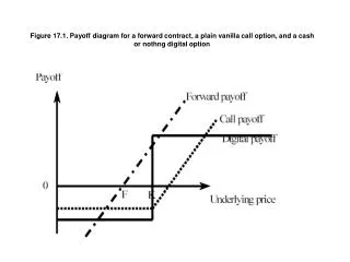
Put-Call Parity • If we accept that there are no arbitrages available in the financial markets, we can use that notion to formulate some basic relationships between calls, puts, the underlying asset, and the risk-free interest rate. • The one we will examine is Put-Call parity. • This is predicated upon the basic notion that a call, put and stock have payout diagrams that look like the following graph.
Put-Call Parity • Put-Call Parity for European Options • This is the most important general relationship between options, the strike price and the underlying asset. • To get at this we once again form two portfolios: • Portfolio A: Call option and cash of Ke-r(T-t) • Portfolio B: Put option and one unit of the underlying. • At time T, these portfolios have the following values: • Portfolio A: • If ST<=K, then let option expire and have cash of $K. • If ST>K, then exercise option, and have underlying with value of ST. • Portfolio B: • If ST<=K, then exercise put and sell underlying for $K. • If ST>K, then let put expire and have stock worth SK.
Put-Call Parity • So, regardless of whether we hold Portfolio A or Portfolio B, we get the same value at time T: • If ST<=K, portfolio=$K. • If ST>K, portfolio = ST. • Since these are European options, if they have the same value at maturity they must have the same value at time t, since you cannot exercise them during the interim. Thus: • PV(A) = PV(B), and since we know the components of both portfolios it must be the case that:c+Ke-r(T-t)= p+St • This is usually written as: • c-p=St-Ke-r(T-t)or c=p+St-Ke-r(T-t)
Put-Call Parity • The condition on the previous slide actually only holds for European options. For American options we have to modify it a bit. • First, for a non-dividend paying underlying, it is never optimal to exercise an American call option early. • You can always sell it in the market for more than its intrinsic value. • In fact, it is generally true that an American call option on a non-dividend paying underlying asset will have the same value as a European option on the same underlying (assuming the same strike, maturity, etc.) • This is generally not true for American put options however. • The reason is that it is sometimes optimal to exercise an American put early. This will happen when the put is very deeply in the money. • It is the fact that you might exercise an American put option early that forces us to modify the put-call parity formula.
Put-Call Parity • Recall the put-call parity relationship for European options: • c + Ke-r(T-t) = p + St • Since we know that P>=p, and that C=c, we can see that when we substitute in the American options, the right side of the equation must be greater than or equal to the left side: • C + Ke-r(T-t) <= P + St