Download
1 / 24
240 likes | 340 Views
FCAL. Collaboration High precision design. LumiCal Optimization Simulations. Iftach Sadeh Tel Aviv University. May 6 th 2008. Performance requirements. X,Y. Z. Compare Angles. Required precision is: Measure luminosity by counting the number of Bhabha events ( N ):. Design parameters.

E N D
FCAL CollaborationHigh precision design LumiCal Optimization Simulations Iftach SadehTel Aviv University May 6th 2008
Performance requirements X,Y Z Compare Angles • Required precision is: • Measure luminosity by counting the number of Bhabha events (N):
Design parameters • 1. Placement: • 2270 mm from the IP • Inner Radius - 80 mm • Outer Radius - 190 mm 2. Segmentation: • 48 azimuthal & 64 radial divisions: • Azimuthal Cell Size - 131 mrad • Radial Cell Size - 0.8 mrad 3. Layers: • Number of layers - 30 • Tungsten Thickness - 3.5 mm • Silicon Thickness - 0.3 mm • Elec. Space - 0.1 mm • Support Thickness - 0.6 mm
Eres(θmax) Eres(θmin) Energy resolution (Eres) / Polar resolution and bias (σ(θ) , Δθ) • Define minimal and maximal polar angles for a shower. σ(θ) Δθ Min{σ(θ)} • Choose constant which minimizes the resolution, σ(θ), but does not necessarily minimizes the bias as well. Min{Δθ}
MIP (muon) Detection • Many physics studies demand the ability to detect muons (or the lack thereof) in the Forward Region. • Example: Discrimination between super-symmetry (SUSY) and the universal extra dimensions (UED) theories may be done by measuring the smuon-pair production process. The observable in the figure, θμ, denotes the scattering angle of the two final state muons. “Contrasting Supersymmetry and Universal Extra Dimensions at Colliders” – M. Battaglia et al. (http://arxiv.org/pdf/hep-ph/0507284)
MIP (muon) Detection • Multiple hits for the same radius (non-zero cell size). • After averaging and fitting, an extrapolation to the IP (z = 0) can be performed. Layer-hit radial positions Averaged radial positions
Induced charge in a single cell • Energy/Charge conversion: • Distribution of the deposited energy spectrum of a MIP (using 250 GeV muons):MPV = 89 keV ~ 3.9 fC. • Distributions of the charge in a single cell for 250 GeV electron showers, and of the corresponding maximal cell signal (for 96 and 64 radial divisions). MIPs Signal distribution Max signal
Digitization Eres σ(θ) Δθ
Number of radial divisions Δθ σ(θ) • Dependence of the polar resolution, bias and subsequent error in the luminosity measurement on the angular cell-size, lθ.
Inner and outer radii antiDID DID • Beamstrahlung spectrum on the face of LumiCal: For the preferable antiDID case Rmin must be larger than 7cm. ( Shown by C.Grah at theOct 2007 FCAL meeting ) 6cm 8cm 19cm
Thickness of the tungsten layers Signal distribution Eres σ(θ) Δθ ( The cut matters! )
Clustering - Event Sample • Bhabha scattering with √s = 500 GeV θ Φ Energy • Separation between photons and leptons: • As a function of the energy of the low-energy-particle (angular distance). • Distribution of the distance (on the face of LumiCal).
Clustering - Algorithm • Phase II:Cluster-merging in a single layer. • Phase I:Near-neighbor clustering in a single layer.
Clustering - Algorithm • Phase III:Global-clustering.
Clustering - Results • Merging-cuts:
Summary • Optimal parameters for the present detector-concept: • [Rmin → Rmax] = [80 → 190] mm → σB = 1.23 nb. • 64 radial divisions (0.8 mrad radial cell-size)→ Δθ = 3.2∙10-3 , σθ = 2.2∙10-2 mrad→ΔL/L = 1.5∙10-4 . • 48 azimuthal → enough for clustering, but shouldn’t be lower… • Tungsten thickness of 3.5 mm → 30 layers are enough for stabilizing the energy resolution at Eres ≈ 0.21 √GeV.
Leakage through the back layers • Distribution of the total energy for a LumiCal of 30 or 90 layers. • (normalized) energy deposited per layer for a 90-layer LumiCal.
Effective layer-radius, reff(l) / Moliere Radius, RM • Dependence of the layer-radius on the layer number, l. r(l) RM RM(layer-gap) • Shower profile - RM is indicated by the red circle.
Clustering - Energy density corrections • Event-by-event comparison of the energy of showers (GEN) and clusters (REC). Before After
Clustering - Results (relative errors) • Dependence on the merging-cuts of the errors in counting the number of single showers which were reconstructed as two clusters (N1→2), and the number of showers pairs which were reconstructed as single clusters, (N2→1).
Clustering - Results (event-by-event) Energy • Event-by-event comparison of the energy and position of showers (GEN) and clusters (REC). θ Φ
Clustering - Results (measurable distributions) Energylow Energyhigh θhigh θlow • Energy and θ of high and low-energy clusters/showers. • Difference in θ between the high and low-energy clusters/showers. Δθhigh,low