Download
1 / 20
200 likes | 311 Views
Attribution of Stratospheric Temperature Trends to Forcings. A coupled chemistry-climate model (CCM) study Richard S. Stolarski NASA GSFC In collaboration with Steven Pawson, Anne Douglass, Paul Newman, Mark Schoeberl and Eric Nielsen.

E N D
Attribution of Stratospheric Temperature Trends to Forcings A coupled chemistry-climate model (CCM) study Richard S. Stolarski NASA GSFC In collaboration with Steven Pawson, Anne Douglass, Paul Newman, Mark Schoeberl and Eric Nielsen SPARC Temperature Trends Meeting, Washington DC, April 12-13, 2007
Difference in Temperature between Past and Future Simulations Past simulation used observed SSTs (1950-2005). Future simulation used model-generated SSTs (1996-2100). Overlap period was used to adjust future temperatures to make a consistent time series. Contours indicate the latitude and altitude dependence of the adjustments. All temperatures used in this analysis are annual means.
Model Simulated Temperature Change 1979-1998(K/decade) Upper Stratospheric Cooling by Radiation to Space Dynamic Response to Ozone Hole Ozone Hole Cooling Tropospheric Warming Can we quantitatively separate the contributions of ozone change and greenhouse gases in our simulations?
Fitting Model Temperature Time Series to EESC, CO2, and CH4 Terms: Midlatitude Upper Stratosphere We will fit this function with 4 terms: Mean + a1•EESC + a2 •CO2 + a3 • CH4
Fitting Model Temperature Time Series to EESC, CO2, and CH4 Terms: Midlatitude Upper Stratosphere Thin line: model output CO2 Term (+mean) Thick line: Fit with All Terms EESC Term (+mean) CH4 Term (+mean) Fit uses entire 140-year simulation time series
Change from 1979-1998 -1.9K EESC -0.7K CO2 -0.4K CH4 -3.0K Total Fitting Model Temperature Time Series to EESC, CO2, and CH4 Terms: Midlatitude Upper Stratosphere Thin line: model output CO2 Term (+mean) Thick line: Fit with All Terms EESC Term (+mean) CH4 Term (+mean)
Change from 1979-1998 -1.9K EESC -0.7K CO2 -0.4K CH4 -3.0K Total Change from 2006-2025 +0.7K EESC -1.3K CO2 -0.6K CH4 -1.2K Total Fitting Model Temperature Time Series to EESC, CO2, and CH4 Terms: Midlatitude Upper Stratosphere Thin line: model output CO2 Term (+mean) Thick line: Fit with All Terms EESC Term (+mean) CH4 Term (+mean)
Relative Contribution of EESC, CO2, and CH4 to Temperature Change at 1 hPa 40oN
How long must the record be to separate effects by time-series analysis?
Effect of Length of Record on Fitting: Graphical Illustration: 40oN, 1hPa
Effect of Length of Record on Fitting: Graphical Illustration: 40oN, 1hPaContinued
Sensitivity to EESC and CO2 as a Function of Endpoint of Output40oN 1hPa These are trends from 1979 through 1998 calculated from output from 1979 through various end years. Thin lines in left panels are .
Northern Mid Latitude Lower Stratosphere 60% EESC Methane term includes effects of increased HOx
Sensitivity to EESC and CO2 as a Function of Endpoint of Output40oN 50hPa Statistically significant after 2020, but uncertainty never gets less than 50%
Fitting Model Temperature Time Series to EESC, CO2, and CH4 Terms: Antarctic Lower Stratosphere Thin line: model output Antarctic lower stratospheric temperature is dominated by ozone hole from ~1960 through 2100. Greenhouse gas terms are minor. Thick line: Fit with All Terms CH4 Term (+mean) CO2 Term (+mean) EESC Term (+mean)
Fitting Model Temperature Time Series to EESC, CO2, and CH4 Terms: Antarctic Upper Stratosphere Antarctic upper stratospheric temperature increases due to dynamic response to ozone hole through 2000. Thereafter, temperature decreases as ozone hole recovers and GHGs continue to cause decrease.
Map of EESC Term Using Output from 1979 to: Color Regions are Statistically Significant 2015 2020 2010 2025 2040 2060
Greenhouse Gas (CO2) Term Using Output from 1979 to: 2010 2015 2020 2025 2040 2060
Some Tentative Conclusions • Simulations indicate about 2/3 of annual temperature trend of upper stratosphere due to ozone decrease • Simulations indicate about 60% of annual temperature trend of lower mid latitude stratosphere due to ozone decrease • Upper stratospheric ozone effect should be able to be separated from greenhouse gas effect with present data: a few more years are needed to reduce uncertainties (of course this assumes a lot about the simulation’s representation of variability and its lack of QBO and solar cycle).