Download
1 / 42
420 likes | 501 Views
Computing for the LHC. Alberto Pace alberto.pace@cern.ch. Experiment data streams. 40 MHz (1000 TB/sec). Level 1 - Special Hardware. 75 KHz (75 GB/sec). Level 2 - Embedded Processors. 5 KHz (5 GB/sec). Level 3 – Farm of commodity CPUs. 100 Hz (300 MB/sec). Data Recording &

E N D
Computing for the LHC Alberto Pace alberto.pace@cern.ch
Experiment data streams 40 MHz (1000 TB/sec) Level 1 - Special Hardware 75 KHz (75 GB/sec) Level 2 - Embedded Processors 5 KHz(5 GB/sec) Level 3 – Farm of commodity CPUs 100 Hz (300 MB/sec) Data Recording & Offline Analysis A typical data stream for an LHC experiment ...
LHC data flows One year of LHC data (~ 20 Km) • The accelerator will run for 10-15 years • Experiments produce about 15 Million Gigabytes (PB) of data each year (about 2 million DVDs!) • LHC data analysis requires a computing power equivalent to ~100,000 of today's fastest PC processors • Requires many cooperating computer centres, as CERN can only provide ~20% of the capacity Concorde (15 Km) Mont Blanc (4.8 Km) Nearly 1 petabyte/week
Computing available at CERN • High-throughput computing based on commodity technology • More than 35000 cores in 6000 boxes (Linux) • 14 Petabytes on 41’000 drives (NAS Disk storage) • 34 Petabytes on 45’000 tape slots CPU Disk Tape
Organized data replication • Grid services are based on middleware which manages the access to computing and storage resources distributed across hundreds of computer centres • The middleware and the experiments’ computing frameworks distribute the load everywhere available resources are found
LCG Service Hierarchy • Tier-1: “online” to the data acquisition process high availability • Managed Mass Storage – grid-enabled data service • Data-heavy analysis • National, regional support Canada – Triumf (Vancouver) France – IN2P3 (Lyon) Germany – Forschunszentrum Karlsruhe Italy – CNAF (Bologna) Netherlands – NIKHEF/SARA (Amsterdam) Nordic countries – distributed Tier-1 Spain – PIC (Barcelona) Taiwan – Academia SInica (Taipei) UK – CLRC (Oxford) US – FermiLab (Illinois) – Brookhaven (NY) • Tier-0: the accelerator centre • Data acquisition & initial processing • Long-term data preservation • Distribution of data Tier-1 centres • Tier-2: ~200 centres in ~35 countries • Simulation • End-user analysis – batch and interactive
LHC Grid Activity • Distribution of work across Tier0 / Tier1 / Tier 2 illustrates the importance of the grid system • Tier 2 contribution is around 50%; > 85% is external to CERN • Data distribution from CERN to Tier-1 sites • Latest run shows that the data rates required for LHC start-up have been reached and can be sustained over long periods http://gridview.cern.ch
CERN as the core point • CERN has the highestrequirements in termsofstorage in the entire LHC computinggrid • All “raw” data mustbestored at CERN ( > 15 PB per year) • All data mustbereplicatedseveraltimesto the Tier1s centres
The Computer centre revolution Today 2005 2007 2006 2004
Key figures CPU Servers Data Base Servers 2.9 MW Electricity and Cooling 270 CPU and disk servers 140 TB (after RAID10) Network routers O(20K) processors Disk Servers Tape Servers and Tape Library 80 Gbits/s 44 000 tapes, 44 PB O(20K) disks, 7.5 PB
Grid applications spinoffs • More than 25 applications from anincreasing number of domains • Astrophysics • Computational Chemistry • Earth Sciences • Financial Simulation • Fusion • Geophysics • High Energy Physics • Life Sciences • Satellite imagery • Material Sciences • ….. Summary of applications report: https://edms.cern.ch/document/722132
Virtual visit to the computer Centre Photo credit to AlexeyTselishchev
Areas of research in Data Management Reliability, Scalability, Security, Manageability
1/4 Arbitrary reliability • Decouple the “Service reliability” from “Hardware reliability” • Generate sufficient error correction scattered on independent storage which allows reconstruction of data from any foreseeable hardware failure • “Dispersed storage” • Use commodity storage (or whatever minimizes the cost) Fixed size M data chunks N error correction chunks checksum
Arbitrary scalability 2/4 • Global namespace but avoid database bottleneck • Options for metatada • Metadata stored with the data but federated asynchronously • Central metadata repository asynchronously replicated locally • Metadata consistency “on demand”
Global access, and Secure 3/4 • Access as a “File system”, using internet protocols • Xroot, NFS 4.1 • Strong authentication, with “Global identities” • (eg: X509 certificates instead of local accounts) • Fine grained authorization • Supporting users aggregations (groups) • Detailed accounting and journaling • Quota
High manageability 4/4 • Data migrates automatically to new hardware, freeing storage marked for retirement • In depth monitoring, with constant performance measurement, and alarm generation • Operational procedures are limited to “no-brainer” box replacement
Storage Reliability • Reliability is related to the probability to lose data • Def: “the probability that a storage device will perform an arbitrarily large number of I/O operations without data loss during a specified period of time”
Reminder: types of RAID • RAID0 • Disk striping • RAID1 • Disk mirroring • RAID5 • Parity information is distributed across all disks • RAID6 • Uses (Reed–Solomon) error correction, allowing the loss of 2 disks in the array without data loss http://en.wikipedia.org/wiki/RAID
Reed–Solomon error correction ? • .. is an error-correcting code that works by oversampling a polynomial constructed from the data • Any k distinct points uniquely determine a polynomial of degree, at most, k − 1 • The sender determines the polynomial (of degree k − 1), that represents the k data points. The polynomial is "encoded" by its evaluation at n (≥ k) points. If during transmission, the number of corrupted values is < n-k the receiver can recover the original polynomial. • Note: only when n-k ≤ 2, we have efficient implementations • n-k = 1 is Raid 5 (parity) • n-k = 2 is Raid 6 http://en.wikipedia.org/wiki/Reed-Solomon
Reed–Solomon (simplified) Example • 4 Numbers to encode: { 1, -6, 4, 9 } (k=4) • polynomial of degree 3 (k − 1): • We encode the polynomial with n=7 points { -2, 9, 8, 1, -6, -7, 4 } y = x3 - 6x2 + 4x + 9
Reed–Solomon (simplified) Example • To reconstruct the polynomial, any 4 points are enough: we can lose any 3 points. • We can have an error on any 2 points that can be corrected: We need to identify the 5 points “aligned” on the only one polynomial of degree 3 possible http://kernel.org/pub/linux/kernel/people/hpa/raid6.pdf
Raid 5 reliability • Disk are regrouped in sets of equal size. If c is the capacity of the disk and n is the number of disks, the sets will have a capacity of c (n-1) example: 6 disks of 1TB can be aggregated to a “reliable” set of 5TB • The set is immune to the loss of 1 disk in the set. The loss of 2 disks implies the loss of the entire set content.
Raid 6 reliability • Disk are regrouped in sets of arbitrary size. If c is the capacity of the disk and n is the number of disks, the sets will have a capacity of c (n-2) example: 12 disks of 1TB can be aggregated to a “reliable” set of 10TB • The set is immune to the loss of 2 disks in the set. The loss of 3 disks implies the loss of the entire set content.
Disks MTBF is between 3 x 10⁵ and 1.2 x 10⁶ hours Replacement time of a failed disk is < 4 hours Probability of 1 disk to fail within the next 4 hours Probability to have a failing disk in the next 4 hours in a 15 PB computer centre (15’000 disks) Imagine a Raid set of 10 disks. Probability to have one of the remaining disk failing within 4 hours However, let’s increase this by two orders of magnitude as the failure could be due to common factors (over temperature, high noise, EMP, high voltage, faulty common controller, ....) Probability to lose computer centre data in the next 4 hours Probability to lose data in the next 10 years Some calculations for Raid 5 p( A and B ) = p(A) * p(B/A) if A,B independent : p(A) * p(B)
Probability of 1 disk to fail within the next 4 hours Imagine a raid set of 10 disks. Probability to have one of the remaining 9 disks failing within 4 hours (increased by two orders of magnitudes) Probability to have another of the remaining 8 disks failing within 4 hours (also increased by two orders of magnitudes) Probability to lose data in the next 4 hours Probability to lose data in the next 10 years Same calculations for Raid 6
Arbitrary reliability s s m n • RAID is “disks” based. This lacks of granularity • For increased flexibility, an alternative would be to use files ... but files do not have constant size • File “chunks” is the solution • Split files in chunks of size “s” • Group them in sets of “m” chunks • For each group of “m” chunks, generate “n” additional chunks so that • For any set of “m” chunks chosen among the “m+n” you can reconstruct the missing “n” chunks • Scatter the “m+n” chunks on independent storage
Arbitrary reliability with the “chunk” based solution • The reliability is independent form the size “s” which is arbitrary. • Note: both large and small “s” impact performance • Whatever the reliability of the hardware is, the system is immune to the loss of “n” simultaneous failures from pools of “m+n” storage chunks • Both “m” and “n” are arbitrary. Therefore arbitrary reliability can be achieved • The fraction of raw storage space loss is n / (n + m) • Note that space loss can also be reduced arbitrarily by increasing m • At the cost of increasing the amount of data loss if this would ever happen
Analogy with the gambling world • We just demonstrated that you can achieve “arbitrary reliability” at the cost of an “arbitrary low” amount of disk space. By just increasing the amount of data you accept loosing when this happens. • In the gambling world there are several playing schemes that allows you to win an arbitrary amount of money with an arbitrary probability. • Example: you can easily win 100 Euros at > 99 % probability ... • By playing up to 7 times on the “Red” of a French Roulette and doubling the bet until you win. • The probability of not having a “Red” for 7 times is (19/37)7 = 0.0094) • You just need to take the risk of loosing 12’700 euros with a 0.94 % probability
Practical comments • n can be 1 or 2 • 1 = Parity • 2 = Parity + Reed-Solomon, double parity • Although possible, n > 2 has a computational impactthat affects performances • m chunks of any (m + n) sets are enough to obtain the information. Must be saved on independent media • Performance can depend on m (and thus on s, the size of the chunks): The larger m is, the more the reading can be parallelized • Until the client bandwidth is reached m n
Reassembling the chunks Data reassembled directly on the client (bittorrent client) Reassembly done by the data management infrastructure Middleware
Identify broken chunks • The SHA1 hash (160 bit digest) guarantees chunks integrity. • It tells you the corrupted chunks and allows you to correct n errors (instead of n-1 if you would not know which chunks are corrupted) s m n Sha1 hash