Download
1 / 56
560 likes | 691 Views
PART 1: CAPITAL STRUCTURE. Prepared by: C. Lamprinoudakis , Ph.D candidate Department of Banking and Financial Management 2009. OUTLINE OF PART 1. Introduction Leading Theories 2.1. Benchmark: MM Irrelevance Propositions 2.2. Trade-off Theory 2.3. Pecking Order Theory

E N D
PART 1: CAPITAL STRUCTURE Prepared by: C. Lamprinoudakis, Ph.D candidate Department of Banking and Financial Management 2009
OUTLINE OF PART 1 • Introduction • Leading Theories 2.1. Benchmark: MM Irrelevance Propositions 2.2. Trade-off Theory 2.3. Pecking Order Theory • Empirical Implications & Evidence 3.1. Leverage Factors 3.2. Tests of the Trade-off 3.3. Tests of the Pecking Order Theory • Summary
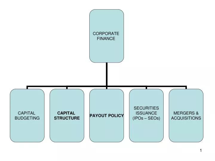
1. INTRODUCTION • Capital Structure is the mix of financial instruments used to finance real investments by corporations. • FUNDAMENTAL QUESTION: Does capital structure matter? • ANSWER: There is no unconditional answer. • Modigliani and Miller set in 1958 the assumptions under which a firm’s value is independent of its capital structure. Their irrelevance proposition is the cornerstone of capital structure theory.
1. INTRODUCTION • The leading theories of capital structure attempt to explain the proportions of financial instruments observed on the right-hand side of corporations’ balance sheets • The main issues that capital structure literature deals with concern the following questions: • How do firms finance their operations? • Which factors influence these choices? • Is it possible to increase the firm value just by changing the mix of securities issued? • Is there an optimal debt-equity combination that maximizes the value of the firm and if so • What is it? • How is it determined?
2.1. MM IRRELEVANCE PROPOSITIONS • Assumptions • No transaction costs • No bankruptcy costs • Firms issue only two types of claims: risk-free debt and equity • Firms and individuals have the same information • Capital markets are complete • Capital markets are competitive (individuals and firms are price takers) • No taxes • Under the above set of assumptions Modigliani and Miller (1958) showed that: • Proposition I: A firm’s total market value is independent of its capital structure • Proposition II: A firm’s cost of equity increases linearly with its debt-equity ratio
2.1. MM IRRELEVANCE PROPOSITIONS Proof of Proposition I • Two firms, which generate the same (random) expected profit X at t=1 • At t=0 firm U is all-equity, firm L has some risk-free debt in its capital structure • r : risk-free interest rate • Ei : market value of firm’s i equity • Di : market value of firm’s i debt • Vi : total market value of firm i, i=L,U • At t=1 • Firm’s L’s debtholders receive rDL • Firm’s L’s equityhholders receive X-rDL • Firm’s U’s equityhholders receive X • The proof relies on a no-arbitrage argument. We will show that we cannot have VU≠VL, since investors can exploit any arbitrage opportunities and eliminate any market value discrepancies.
2.1. MM IRRELEVANCE PROPOSITIONS • Suppose VL>VU • Suppose an investor owning eL dollars’ worth of the shares of firm L, representing a fraction α of the total shares. • At t=1 he would receive an income • Now suppose the investor sold his αΕL worth of firm’s L shares, borrowed an additional amount αDL and acquired an amount eU=α(EL+DL) of firm’s U shares. • At t=1 his income would be • Since VL>VU , we must have YU >YL (arbitrage profit) → Levered firms cannot command a premium over unlevered firmsbecause investors have the opportunity of putting the equivalentleverage into their portfolio directly by borrowing on personal account (homemade leverage)
2.1. MM IRRELEVANCE PROPOSITIONS • Suppose VU>VL • Suppose an investor owning eU dollars’ worth of the shares of firm U, representing a fraction α of the total shares. • At t=1 he would receive an income • Now suppose the investor sold his eU worth of firm’s U shares and acquired an amount eL=eU(EL/VL) of firm’s L shares and an amount of dL=eU(DL/VL) • At t=1 his income would be • Since VU>VL , we must have YL >YU (arbitrage profit) → Unlevered firms cannot command a premium over levered firms, because investors can undo firm’s Lleverage by buying its debt and equity in proportions such that interest paid and received cancels out.
2.1. MM IRRELEVANCE PROPOSITIONS • Interpretation of Proposition 1 • Consider this market-value balance sheet. P1 says that V is a constant regardless of the proportions of D and E, provided that A are held constant. • When a firm chooses a certain proportion of debt and equity to finance its assets, all it does is to divide up the cash flows among investors. It just divides the “pie” between different claimholders. The size of the ‘pie” does not change. • Firm value is determined on the left-hand side of the balance sheet by real assets – not by the proportions of debt and equity securities issued to buy the assets. • P1 applies for any finite number of securities, not just debt vs. equity (value additivity principle, PV(A) + PV(B) = PV(A+B))
2.1. MM IRRELEVANCE PROPOSITIONS • Proposition 2 is an implication of Proposition 1. Since the market value of a firm is independent of its debt-equity ratio, so is its WACC. • By rearranging the WACC formula we get: Hence rE increases (since WACC > rf ) linearly (since WACC and rf independent of D/E) with D/E.
2.1. MM IRRELEVANCE PROPOSITIONS • Intuition of Proposition 2: More debt makes equity riskier and so increases its cost. When risk-free debt is added to the capital structure, total risk of the firm remains constant. However, debtholders receive part of the cash flows without taking up any risk. That means, that equityholders take up more risk per unit of cash flow and therefore require a higher return. • Proposition 2 goes through even with risky debt, but the relationship is no more linear.
2.1. MM IRRELEVANCE PROPOSITIONS • MM propositions should be thought of as benchmarks, not end results. • They certainly don’t generate realistic predictions of how firms finance their operations, but they provide a means of finding reasons of why financing may matter. • If we can identify the conditions under which capital structure is irrelevant, we may able to infer what makes it relevant. • The main theories that dominate capital structure literature until today were developed by relaxing one or more assumptions that generate MM propositions.
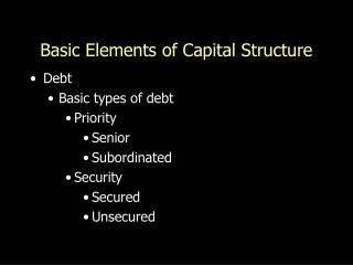
2.2. TRADE-OFF THEORY • STATIC TRADE OFF THEORY A firm is said to follow the static trade-off theory if the firm’s leverage is determined by the trade-off between the tax benefits of debt and the expected costs of bankruptcy. • Use of debt has both costs and benefits for the firm: • Benefit: debt has a tax advantage over equity • Cost: debt creates the possibility of costly bankruptcy • MM assumptions for corporate taxes and bankruptcy costs are relaxed
2.2. TRADE-OFF THEORY Benefits of debt • MM (1963) introduced corporate income taxes into Proposition 1. Interest payments on debt are tax deductible, while dividend and retained earnings are taxed. • Consider a firm that: • generates (random) cash flow X • has a constant amount of risk-free debt D in perpetuity • τc is the corporate tax rate • rf is the risk free rate • VU is the value of an unlevered firm generating the same cash flows • Each period the after tax cash flow to all claimholders is: (cash flow to equityholders + cash flow to debtholders)
2.2. TRADE-OFF THEORY • By rearranging we get: (cash flow to equityholders of unlevered firm + tax shield) • Assuming perpetuity, the value of the levered firm is: • MM Proposition with Corporate Taxes (1963): The value of a levered firm equals the sum of the value of an unlevered firm and the PV of the interest tax shield
2.2. TRADE-OFF THEORY Costs of Debt • Corporate bankruptcies occur when stockholders exercise their right to default. It is a legal mechanism allowing creditors to take over when the firm defaults. Bankruptcy costs are the costs of using this mechanism • Direct bankruptcy costs • Administrative and court costs • Lawyers, accountants and advisors fees • Time and resources spent by management and creditors dealing with bankruptcy • Indirect bankruptcy costs • Loss of intangible assets (brand name, reputation) • Loss of key employees, suppliers, customers • Constraint capital investments (positive NPV projects may be passed up) • Fire sale of assets (below their replacement value)
2.2. TRADE-OFF THEORY • An increase in the debt level has two effects: • as D increases, the PV of the tax shield and so the firm value increases • as D increases the probability of bankruptcy increases and hence the expected bankruptcy costs (= probability of bankruptcy x estimated bankruptcy costs) increase • That is, (Static Trade-off formula) • At the optimum debt level: Marginal increase in PV of the Tax Shield = Marginal increase in Expected Bankruptcy Costs • This optimal debt ratio becomes the firm’s target debt-equity ratio, often referred to as debt capacity. This theory suggest that firms keep a relatively constant debt-equity ratio.
2.2. TRADE-OFF THEORY • This model gives a solution for leverage, but it leaves no room for the firm to be anywhere but at the solution. Since rebalancing is costless, firms should react to adverse shocks immediately. • Costly adjustment (Dynamic Trade-off): Because of transaction costs, firms allow their leverage to drift within a range around the optimal leverage ratio and rebalance only when the benefits of adjustment to the target are likely to exceed the costs. • This implies that actual debt ratios should have a mean-reverting behavior around target ratios.
2.3. PECKING ORDER THEORY • MM assumption about firms and individuals having the same information is relaxed • Key idea: Owners/managers of firms know more about their firms’ prospects, risk and values than outside investors do. This asymmetric information generates adverse selection problems when firms turn to external financing. • Implications: • Securities issued by firms are mispriced (adverse selection cost) • Some firms do not undertake positive NPV investment projects • Low quality firms (in terms of risk and profitability of their investments projects) are more likely than high quality firms to get funded • Financing choices can eliminate or mitigate adverse selection costs. Hence capital structure matters under asymmetric information.
2.3. PECKING ORDER THEORY • PECKING ORDER THEORY: • A firm is said to follow the pecking order theory if it prefers internal (retained earnings) to external financing and debt to equity if external financing is used. Equity is used only as a last resort. • The idea is that good firms should issue securities whose value is at least information sensitive because they are least underpriced (adverse selection cost). • According to this theory, firms do not have a target debt-equity ratio, since there are two kinds of equity, internal and external, one at the top of the pecking order and one at the bottom. Each firm’s observed ratio reflects its cumulative requirement for external financing.
EMPIRICAL IMPLICATIONS & EVIDENCE Some general comments about empirical research • The theories of capital structure implicitly assume that firms have access to broad, efficient capital markets and to modern financial institutions. • Therefore, most empirical papers use samples of established, public USA corporations (financial firms and regulated utilities excluded) in order to test capital structure theories. • Even in that well-structured setting evidence is quite often contradictory to theories. Myers (2003, p. 247) argues that “….export of theories may therefore seem premature and foolhardy.”
3.1. LEVERAGE FACTORS • This strand of literature is concerned with determining which factors are correlated in the cross-section with firm leverage. • These papers are not definitive tests of any theory. Rather they provide evidence on the patterns of the data. • However, by interpreting the theories one can infer predictions for some of the factors. • The regression usually used to study the effects of the factors is: • : market leverage (total debt divided by the sum of total debt and market value of equity) of firm i on date t • : set of factors observed at firm i on date t-1
3.1. LEVERAGE FACTORS • Empirical research (Harris and Raviv JF 1991, Rajan and Zingales JF 1995, Fama and French RFS 2002, Frank and Goyal WP 2007) has settled on a few factors that account for much of the variation in leverage across firms (almost 30%): • Growth opportunities (-) • Firm size (+) • Tangibility of assets (+) • Profitability (-) • Median industry leverage (+) • Large firms with tangible assets tend to borrow more than small with intangible assets. • Firms with high profitability and/or valuable investment opportunities borrow less. • Firms in the same industry face common forces that seem to affect their financing decisions.
3.1. LEVERAGE FACTORS • How do these factors relate to theory (predictions about leverage)
Dynamic tradeoff hypothesis • Firms do not adjust their leverage ratios constantly because of transaction costs. Instead, they allow leverage ratios to move within a range around the optimal target ratios. Within this range, the market equity values of more profitable firms grow faster, leading to the negative relation between profitability and leverage ratios. When resorting to external funds (i.e., when the adjustment boundaries are reached), more profitable firms are more likely to issue debt relative to equity in an effort to move toward their target ratios. In a nutshell, a negative relation between profitability and leverage ratio may exist because some (profitable) firms temporarily deviate from their target ratios. • In any case, the costly adjustment argument predicts that the combination of debt and equity must be in the direction of correcting the deviations from the target ratios.
3.1. LEVERAGE FACTORS • Summarizing: • Empirical evidence on leverage factors is consistent with the predictions of trade-off theory (3 out of 4 factors for the static version and the remaining factor – profitability – consistent with the dynamic version). • Pecking order predicts only the profitability factor correctly. The other predictions are either inconsistent with empirical evidence or ambiguous.
3.2. TRADE-OFF TESTS COST AND BENEFITS OF DEBT • This strand of literature tests the static trade-off theory. • Relevant studies attempt to quantify: • expected bankruptcy costs • tax benefits of debt
3.2. TRADE-OFF TESTS Bankruptcy Costs • Warner (JF, 1977) examines 11 bankrupt US railroads and reports direct costs between 1% (7 years before bankruptcy) and 5% (when entering bankruptcy) of the firm market value. • Weiss (JFE, 1990) studies 37 public US firms that went bankrupt and finds costs of 3,1% of firm market value (at the fiscal year-end before entering bankruptcy). • Andrade & Kaplan (JF, 1998) study 31 firms that went bankrupt and estimate the sum of direct and indirect costs to be between 10% and 20% of firm value. (indirect costs are measured as the decline in operating margins – EBITDA/sales – from the first year that a firm reports EBITDA lower than interest expenses to the first year after bankruptcy resolution)
3.2. TRADE-OFF TESTS • Remember: Expected bankruptcy costs = Probability of bankruptcy × Estimated bankruptcy costs as % of firm value • In all cases, these numbers overestimate the relevant costs, because the firm value is especially low close to bankruptcy. • Besides, in the trade-off theory framework, the relevant cost is the expected cost of financial distress, which is the estimated cost multiplied by the probability of distress. Since the probability of distress is very small for firms operating at normal debt ratios, the expected financial distress costs will also be very low.
3.2. TRADE-OFF TESTS Tax benefits • Graham (JF, 2000) examined a sample of US public firms. He estimated that the tax-reducing benefit was 10% of firm value on average. • However, these firms were highly profitable and operating in stable industries. That means that they were facing a remote probability of financial distress. Therefore, Graham argues that they could lever up to still conservative debt ratios without being threatened by financial distress (7.5% of firm value mean incremental net benefit). • Assuming that the new ratios would be optimal in a trade-off perspective and using Andrade and Kaplan (JF, 1998) estimates of bankruptcy costs, the implied default probabilities lie between 33% and 75%. Corporate bond default rates of issuers comparable to those in Graham’s sample range between 0.4 and 7.2%.
3.2. TRADE-OFF TESTS • Summarizing • Empirical studies indicate that many firms use debt conservatively: they have lower leverage than would maximize firm value from a static trade-off perspective. • Besides, profitable firms which could have issued a large amount of debt, while still having a (practically) zero probability of bankruptcy, do not issue debt at all (the “Microsoft Paradox”).
3.2. TRADE-OFF TESTS • Some attempts to reconcile observed debt ratios with those predicted by static trade-off theory: • Agency costs of debt (Parino & Weisbach 1999) • Low leverage is temporary: firms with low leverage appear to be stockpiling financial slack or debt capacity, which is used later to make capital expenditures or acquisitions (Minton & Wruck, 2001) • Tax shelters (Graham & Tucker, 2006)
3.2. TRADE-OFF TESTS MEAN REVERSION OF LEVERAGE • Trade-off theory predicts a target debt ratio that depends on the tax benefits of debt and the bankruptcy costs. • The dynamic version predicts that due to transaction costs firms allow their leverage to drift until rebalancing benefits outweigh its costs. Hence, firms allow leverage to move within a range surrounding the optimal leverage ratio and rebalance when the boundaries of this range are reached. • This translates to the empirical hypothesis that actual debt ratios will revert towards an optimum/target level. • This strand of literature focus on two related questions: • Does firm-level leverage revert to a target? • If so, how rapidly does this adjustment take place?
3.2. TRADE-OFF TESTS • In order to test for mean reversion, a two step procedure is adopted (some recent papers adopt a one-step procedure with direct substitution): • first, an equation for the target leverage is estimated • : leverage of firm i in year t • : set of firm characteristics (assumed to determine optimal leverage) in year t-1 • : vector of parameters to be estimated • then, the fitted value is substituted into the partial adjustment equation • : is the predicted target leverage obtained form target equation • : is the speed of adjustment
3.2. TRADE-OFF TESTS • A positive and significant λ implies that leverage is mean-reverting. For example, an estimated value of 0.65 implies that firms close on average 65% of the gap between current and desired leverage per year. The closer it is to 1, the more full is the adjustment. • The existence of a leverage target and the speed of adjustment towards the target have become topics of intense debate and are considered currently the most important issues in capital structure research:
3.2. TRADE-OFF TESTS • Question 1: Is there a target? Answer: Yes, the literature agrees that leverage exhibits mean reversion (all studies report positive and significant coefficients across different variable specifications, econometric techniques and robustness checks). • Question 2: How fast is this adjustment? Answer: Not a settled issue yet (sensitive to different variable specification and econometric procedures): • Slow FF 2002: 7-18%, HR 2007: 11-21% • Fast FR 2006: 34-36%, LR 2005: 33-50% The second question is very important: • If adjustment speed is low (implying that it takes an average firm many years to offset the initial deviation from the target), then target leverage should be viewed as a secondary factor in corporate financing decisions. • If adjustment is fast, then target leverage is of central importance
3.2. TRADE-OFF TESTS • The latest step of the literature concerning the second question is to try to identify cross-sectional variation in adjustment costs and test whether such costs are correlated with capital structure activities. Higher adjustment cost should be associated with slower movements towards target leverage and vice versa (3 latest papers): • Faulkender et al (WP, 2007): They argue that firms which incur very positive or very negative cash flow outcomes face lower adjustment costs than firms with cash flow outcome close to zero: • Negative cash flows: since firms are likely to raise funds anyway (to cover their financial deficit), they can choose securities that they will move them toward target leverage • Positive cash flows: paying dividends or paying down debt are relatively inexpensive adjustment mechanisms They find that adjustment speeds approaching 50% on average for years in which firms face substantial financial deficits or surpluses compared to just 25% for years in which firms have cash flow realizations close to 0.
3.2. TRADE-OFF TESTS • Hovakimian and Li (WP, 2008) They argue that firms have the opportunities to adjust at low marginal costs: • when long-term debt is maturing • when firms initiate more than one type of transaction (e.g. issue both debt and equity, issue debt and repurchase equity) The intuition is that since firms engage in financing transactions anyway, the incremental cost of doing so in a manner that allows them to adjust to the target should be low, especially in cases of dual transactions. They find an average speed of adjustment of 20%. The speed in the other two special cases is higher (30%) but far less than 1.
3.2. TRADE-OFF TESTS • Byoun (JF, 2008) Since the transaction costs (flotation costs) are higher for equity than for debt, we should expect that : • when firms face a financial deficit, the speed of adjustment will be faster when firms have below target debt (cheaper to issue debt than equity) • when firms have a financial surplus, the speed of adjustment will be faster when firms have above target debt (more willing to reduce debt than equity, in order to preserve debt capacity for future financing needs) They find the following speeds: • conditional on financial surpluses: 33% when firms have above target debt vs 5% when firms have below target debt and • conditional on financial deficits: 20% when firms have below target debt vs 2% when firms have above target debt.
3.2. TRADE-OFF TESTS • Summarizing • The literature commonly agrees that leverage is mean-reverting at the firm level. • However, the speed at which this happens is not a settled issue. • Concerning cross-sectional variation in adjustment costs, the first evidence implies that: • adjustment costs do affect financing activities, but • adjustment is not full (not even close), even in cases that should be, if transaction costs were the only impediment
3.4. PECKING ORDER TESTS • The pecking order model says that when a firm’s internal cash flows are not enough for its real investments and dividend commitments, the firm issues debt. Equity is never issued, except when the firm can only issue junk debt and costs of financial distress are high. • This translates to the empirical hypothesis that debt ratios are driven by the financing deficit of the firm.
3.4. PECKING ORDER TESTS • Shyam-Sunder and Myers (JFE, 1999) use a sample of 157 large public US firms for the period 1971-1989. • The financing deficit is defined as Ct= operating cash flows, after interest and taxes DIVt= dividend payments Xt=capital expenditure ΔWt = net increase in working capital
3.4. PECKING ORDER TESTS • The pecking order hypothesis to be tested is: where ΔDit is the amount of debt issued (or retired if DEFit is negative) by firm i in year t. • The theory predicts that a = 0 and bPO = 1. The slope coefficient indicates the extent to which new debt issues (retirements) are explained by financing deficits (surpluses). • A semi-strong form of Pecking Order hypothesis implies that bPO will be less than but close to unity.
3.4. PECKING ORDER TESTS • SS & M find strong support for this prediction. For net debt issues (issues – retirements) the coefficient bPO is found to be 0,75 with an of 0,68. • They interpret this evidence to imply that “…pecking order is an excellent first order descriptor of corporate financing behavior” (SS & M 1999, p.242) • However, subsequent papers disputed the results. • Chirinco and Singha (JFE, 2000) low power of statistical test • Frank and Goyal (JFE, 2003) incomplete sample
3.4. PECKING ORDER TESTS Chirinco and Singha (JFE, 2000) • The key empirical prediction of the Pecking Order hypothesis is about ordering: equity issues, if they occur at all, are at the bottom of the financial hierarchy. • The method proposed by SS & M tests jointly the ordering (debt comes before equity) and the proportions (equity issues constitute a low percentage of external finance). • They show that: • The slope coefficient can be far less than one for a firm that follows the pecking order but the equity financing is a substantial percentage of overall external finance. (PO rejected when true) • The slope coefficient can be close to unity when (i) a firm issues first equity and then debt or (ii) issues debt and equity in fixed proportionsbut the debt is a substantial percentage of overall external finance (PO not rejected when false)