Download
1 / 24
250 likes | 397 Views
Earth Systems Science Chapter 6. I. Modeling the Atmosphere-Ocean System. Statistical vs physical models; analytical vs numerical models; equilibrium vs dynamical models finite difference vs spectral models endogenous vs exogenous variables

E N D
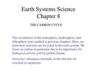
Earth Systems ScienceChapter 6 I. Modeling the Atmosphere-Ocean System • Statistical vs physical models;analytical vs numerical models;equilibrium vs dynamical modelsfinite difference vs spectral modelsendogenous vs exogenous variables • Physically based climate models of different complexities (largely review from discussion in chapter 3) • Global Climate Models (GCMs)
Statistical v Physical Models Statistical Model Based on observations, you identify a relationship between two variables. You do not necessarily understand the reason why this relationship exists. Physical Model Based on the rules of physics, you construct a model that describes the relationships between different physical phenomena.
Numerical vs Analytical Models Analytical Model Equations are solved without the aid of the computer, resulting in one or more equations that allow one to calculate the answer for any time, without calculating each time step (usually using calculus). Complicated, highly non-linear equations often have no analytical solutions. Numerical Model Equations are solved at each time step, usually by computer (STELLA solves numerical models). Can solve any set of equations, regardless of non-linearities.
Equilibrium vs Dynamical Models Equilibrium Model Model that provides solution only for the equilibrium values; solution does not vary as a function of time. Dynamical Model Model that provides solution as a function of time (STELLA solves dynamical models).
Finite Difference vs Spectral Models Finite Difference Model Numerical model in which the calculations are performed in each grid box. Spectral Model Model that uses different mathematical techniques, and performs calculations using wave functions.
Endogenous vs Exogenous Variables Endogenous Variables whose values are calculated as part of the model Exogenous Variables whose values are specified by the modeler Excluded Variables that are not part of the model in any way
Physically-based climate models of different complexities • Many types of climate models exist. We discuss some of the more common types, which have different levels of complexity: • Zero-dimensional radiation balance models • 1-dimensional radiative-convective models • 2-dimensional diffusive models • 3-dimensional Atmospheric General Circulation Models (AGCM) • 3-D coupled atmosphere – ocean models (AOGCM)
SWout SWin LWout Earth’sEnergy Physically-based climate models:zero-dimensional radiation balance model Equilibrium model:Te = [ (S/4s) (1-A) ]0.25
Physically-based climate models:1-dimensional radiative-convective model One-Layer Radiation Model
1-D Rad-Conv Model S/4 (S/4)*A Radiation in each wavelength band surface Physically-based climate models:1-dimensional radiative-convective model Convection, latent fluxes Surface: latent, sensible
North Pole South Pole Surface Physically-based climate models:2-dimensional climate model, or 2-d energy balance model (EBM)
Physically-based climate models:3-dimensional Atmospheric General Circulation Model (AGCM) surface http://www.arm.gov/docs/documents/project/er_0441/bkground_5/figure2.html
Atmosphere Flux adjustment Ocean Physically-based climate models:3-D coupled atmosphere – ocean general circulation models(AOGCM) or Global Climate Model (GCM)
I. Global Climate Models • processes • Climate change experiments- equilibrium- transient • Model resolution, subgrid-scale processes • Dependency on initial conditions • Results from different models
Global Climate Models (GCMs): many processes Boundary conditions (exogenous variables) vs modeled processes (endogenous variables)
Included in Climate Model Separate Models
Climate Change Experiments Typically, experiments are performed using climate models (usually GCMs) to estimate the effect of changing boundary conditions (e.g. increasing carbon dioxide) on climate. Control Run Model experiment simulating current climate conditions using current boundary conditions (e.g. CO2) Equilibrium experiments Model experiment simulating the climate under changed conditions by changing the boundary conditions to what they might be at some future time (e.g. doubled CO2, or 2xCO2) Transient Experiments Model experiment simulating the gradual change from current to future (e.g. increase in CO2 by 1% per year)
Transient Experiments Figure 9.1: Global mean temperature change for 1%/yr CO2 increase with subsequent stabilisation at 2xCO2 and 4cCO2. The red curves are from a coupled AOGCM simulation (GFDL_R15_a) while the green curves are from a simple illustrative model with no exchange of energy with the deep ocean. The “transient climate response”, TCR, is the temperature change at the time of CO2 doubling and the “equilibrium climate sensitivity”, T2x, is the temperature change after the system has reached a new equilibrium for doubled CO2, i.e., after the “additional warming commitment” has been realised. http://www.grida.no/climate/ipcc_tar/wg1/345.htm#fig91
Model Resolution & subgrid scale processes resolution How big are the grid boxes? The larger they are, the less realistic the model; typically ~1 degree lat/lon.Bigger grid boxes = lower resolutionSmaller grid boxes = higher resolution Subgrid-scale processes many physical processes that are important for climate occur on very small spatial scales (e.g. cloud formation). Since the model resolution is much larger, these processes can not be modeled “physically” parameterization a simple method, usually a statistical model, to account for subgrid-scale processes for which the physically-based equations can not be included.
Dependency on Initial Conditions Initial conditions the values of all “stocks” or “state variables” (e.g. temperature, pressure, etc) at each grid point must be specified in the beginning of a model experimentThe transient response of GCMs can change when initial conditions are changed even slightly. This is because the climate is a chaotic system. Ensemble experiments the same model experiment is performed a number of times with slightly different initial conditions; the results of the ensemble members are averaged to get the “ensemble mean”
Dependency on Initial Conditions Figure 9.2: Three realisations of the geographical distribution of temperature differences from 1975 to 1995 to the first decade in the 21st century made with the same model (CCCma CGCM1) and the same IS92a greenhouse gas and aerosol forcing but with slightly different initial conditions a century earlier. The ensemble mean is the average of the three realisations. (Unit: °C). http://www.grida.no/climate/ipcc_tar/wg1/346.htm#9221
Results from different models Different GCMs have many similarities, and therefore provide, in many ways, similar results. However, the way the different modeling groups choose to parameterize different processes makes the models different. Therefore, the different models produce somewhat different results. For example, the models agree much more closely on temperature than on precipitation. This is because temperature changes are more dependent on large scale processes, which are modeled similarly in most models. Precipitation, however, depends on subgrid-scale processes, which are parameterized differently by the different modeling groups.
Results from different models Figure 9.5: (a) The time evolution of the globally averaged temperature change relative to the years (1961 to 1990) of the DDC simulations (IS92a). G: greenhouse gas only (top), GS: greenhouse gas and sulphate aerosols (bottom). The observed temperature change (Jones, 1994) is indicated by the black line. (Unit: °C). http://www.grida.no/climate/ipcc_tar/wg1/350.htm
Results from different models Figure 9.5: (b) The time evolution of the globally averaged precipitation change relative to the years (1961 to 1990) of the DDC simulations. GHG: greenhouse gas only (top), GS: greenhouse gas and sulphate aerosols (bottom). (Unit: %). http://www.grida.no/climate/ipcc_tar/wg1/350.htm