Download
1 / 32
320 likes | 323 Views
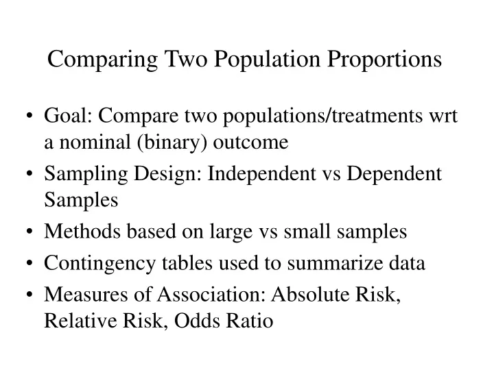
Comparing Two Population Proportions. Goal: Compare two populations/treatments wrt a nominal (binary) outcome Sampling Design: Independent vs Dependent Samples Methods based on large vs small samples Contingency tables used to summarize data

E N D
Comparing Two Population Proportions • Goal: Compare two populations/treatments wrt a nominal (binary) outcome • Sampling Design: Independent vs Dependent Samples • Methods based on large vs small samples • Contingency tables used to summarize data • Measures of Association: Absolute Risk, Relative Risk, Odds Ratio
Contingency Tables • Tables representing all combinations of levels of explanatory and response variables • Numbers in table represent Counts of the number of cases in each cell • Row and column totals are called Marginal counts
Outcome Present Outcome Absent Group Total Group 1 X1 n1-X1 n1 Group 2 X2 n2-X2 n2 Outcome Total X1+X2 (n1+n2)-(X1+X2) n1+n2 2x2 Tables - Notation
High Quality Low Quality Group Total Not Integrated 33 55 88 Vertically Integrated 5 79 84 Outcome Total 38 134 172 Example - Firm Type/Product Quality • Groups: Not Integrated (Weave only) vs Vertically integrated (Spin and Weave) Cotton Textile Producers • Outcomes: High Quality (High Count) vs Low Quality (Count) Source: Temin (1988)
Notation • Proportion in Population 1 with the characteristic of interest: p1 • Sample size from Population 1: n1 • Number of individuals in Sample 1 with the characteristic of interest: X1 • Sample proportion from Sample 1 with the characteristic of interest: • Similar notation for Population/Sample 2
Example - Cotton Textile Producers • p1 - True proportion of all Non-integretated firms that would produce High quality • p2 - True proportion of all vertically integretated firms that would produce High quality
Notation (Continued) • Parameter of Primary Interest: p1-p2, the difference in the 2 population proportions with the characteristic (2 other measures given below) • Estimator: • Standard Error (and its estimate): • Pooled Estimated Standard Error when p1=p2=p:
Cotton Textile Producers (Continued) • Parameter of Primary Interest: p1-p2, the difference in the 2 population proportions that produce High quality output • Estimator: • Standard Error (and its estimate): • Pooled Estimated Standard Error when p1=p2=p:
Confidence Interval for p1-p2 (Wilson’s Estimate) • Method adds a success and a failure to each group to improve the coverage rate under certain conditions: • The confidence interval is of the form:
Example - Cotton Textile Production 95% Confidence Interval for p1-p2: Providing evidence that non-integrated producers are more likely to provide high quality output (p1-p2 > 0)
Significance Tests for p1-p2 • Deciding whether p1=p2 canbe done by interpreting “plausible values” of p1-p2 from the confidence interval: • If entire interval is positive, conclude p1 > p2 (p1-p2 > 0) • If entire interval is negative, conclude p1 < p2 (p1-p2 < 0) • If interval contains 0, do not conclude that p1 p2 • Alternatively, we can conduct a significance test: • H0: p1 = p2Ha: p1 p2 (2-sided) Ha: p1 > p2 (1-sided) • Test Statistic: • P-value: 2P(Z|zobs|) (2-sided) P(Z zobs) (1-sided)
Example - Cotton Textile Production Again, there is strong evidence that non-integrated performs are more likely to produce high quality output than integrated firms
Measures of Association • Absolute Risk (AR): p1-p2 • Relative Risk (RR): p1 / p2 • Odds Ratio (OR): o1 / o2 (o = p/(1-p)) • Note that if p1 = p2 (No association between outcome and grouping variables): • AR=0 • RR=1 • OR=1
Relative Risk • Ratio of the probability that the outcome characteristic is present for one group, relative to the other • Sample proportions with characteristic from groups 1 and 2:
Relative Risk • Estimated Relative Risk: 95% Confidence Interval for Population Relative Risk:
Relative Risk • Interpretation • Conclude that the probability that the outcome is present is higher (in the population) for group 1 if the entire interval is above 1 • Conclude that the probability that the outcome is present is lower (in the population) for group 1 if the entire interval is below 1 • Do not conclude that the probability of the outcome differs for the two groups if the interval contains 1
Example - Concussions in NCAA Athletes • Units: Game exposures among college socer players 1997-1999 • Outcome: Presence/Absence of a Concussion • Group Variable: Gender (Female vs Male) • Contingency Table of case outcomes: Source: Covassin, et al (2003)
Example - Concussions in NCAA Athletes There is strong evidence that females have a higher risk of concussion
Odds Ratio • Odds of an event is the probability it occurs divided by the probability it does not occur • Odds ratio is the odds of the event for group 1 divided by the odds of the event for group 2 • Sample odds of the outcome for each group:
Odds Ratio • Estimated Odds Ratio: 95% Confidence Interval for Population Odds Ratio
Odds Ratio • Interpretation • Conclude that the probability that the outcome is present is higher (in the population) for group 1 if the entire interval is above 1 • Conclude that the probability that the outcome is present is lower (in the population) for group 1 if the entire interval is below 1 • Do not conclude that the probability of the outcome differs for the two groups if the interval contains 1
Osteoarthritis in Former Soccer Players • Units: 68 Former British professional football players and 136 age/sex matched controls • Outcome: Presence/Absence of Osteoathritis (OA) • Data: • Of n1= 68 former professionals, X1 =9 had OA, n1-X1=59 did not • Of n2= 136 controls, X2 =2 had OA, n2-X2=134 did not Interval > 1 Source: Shepard, et al (2003)
Fisher’s Exact Test • Method of testing for association for 2x2 tables when one or both of the group sample sizes is small • Measures (conditional on the group sizes and number of cases with and without the characteristic) the chances we would see differences of this magnitude or larger in the sample proportions, if there were no differences in the populations
Example – Echinacea Purpurea for Colds • Healthy adults randomized to receive EP (n1.=24) or placebo (n2.=22, two were dropped) • Among EP subjects, 14 of 24 developed cold after exposure to RV-39 (58%) • Among Placebo subjects, 18 of 22 developed cold after exposure to RV-39 (82%) • Out of a total of 46 subjects, 32 developed cold • Out of a total of 46 subjects, 24 received EP Source: Sperber, et al (2004)
EP/Cold Plac/Cold 14 18 13 19 12 20 11 21 10 22 Example – Echinacea Purpurea for Colds • Conditional on 32 people developing colds and 24 receiving EP, the following table gives the outcomes that would have been as strong or stronger evidence that EP reduced risk of developing cold (1-sided test). P-value from SPSS is .079.
McNemar’s Test for Paired Samples • Common subjects being observed under 2 conditions (2 treatments, before/after, 2 diagnostic tests) in a crossover setting • Two possible outcomes (Presence/Absence of Characteristic) on each measurement • Four possibilities for each subjects wrt outcome: • Present in both conditions • Absent in both conditions • Present in Condition 1, Absent in Condition 2 • Absent in Condition 1, Present in Condition 2
McNemar’s Test for Paired Samples • H0: Probability the outcome is Present is same for the 2 conditions • HA: Probabilities differ for the 2 conditions (Can also be conducted as 1-sided test)
Example - Juveniles Tried as Adults • Subjects - 2097 pairs of juveniles matched on prior criminal record and severity of current crime • Condition: Adult vs Juvenile Court (one of each in pair) • Outcome: Whether juvenile was re-arrested during follow-up Source: Bishop et al (1996)
Example - Juveniles Tried as Adults • H0: Tendency to for rearrest is not different between children tried as adults as those tried as juveniles • HA: Tendencies differ Evidence that tendencies differ (higher risk of rearrest among juveniles tried in adult court)
Data Sources • Temin, P. (1988). “Product Quality and Vertical Integration in the Early Cotton Textile Industry,” The Journal of Economic History, 48(4), pp891-907 • Covassin, T., C.B. Swanik, and M.L. Sachs (2003). “Sex Differences and the Incidence of Concussions Among Collegiate Athletes,” Journal of Athletic Training, 38(3) pp238-244. • Shepard, G.J., A.J. Banks, and W.G. Ryan (2003). “Ex-Professional Association Footballers Have an Increased Prevalence of Osteoarthritis of the Hip Compared with Age Matched Controls Desite Not Having Sustained Notable Hip Injuries,” British Journal of Sports Medicine, 37, pp80-81. • Sperber, S.J., L.P. Shah, R.D. Gilbert, et al (2004). “Echinacea purpurea for Prevention of Experimental Rhinovirus Colds,” Clinical Infectious Diseases, 38, pp1367-1371. • Bishop,D.M, C.E. Frazier, L. Lanza-Kaduce, L. Winner (1996). “The Transfer of Juveniles to Criminal Court: Does it Make a Difference?” Crime & Delinquency, 42, pp171-191.