Download
1 / 19
230 likes | 508 Views
Princess Nora University. Modeling and Simulation Random Number Generators. Arwa Ibrahim Ahmed. RANDOM NUMBER GENERATORS. The usefulness of these programs is limited by amount of available data: • What if more data needed? • What if the model changed?

E N D
Princess Nora University Modeling and Simulation Random Number Generators Arwa Ibrahim Ahmed
RANDOM NUMBER GENERATORS • The usefulness of these programs is limited by amount of available data: • What if more data needed? • What if the model changed? • What if the input data set is small or unavailable? • A random number generator address all problems It produces real values between 0.0 and 1.0 The output can be converted to random variable via mathematical transformations. • Historically there are three types of generators. • table look-up generators • hardware generators • algorithmic (software) generators
RANDOM NUMBER GENERATORS • algorithmic (software) generators : • Algorithmic generators are widely accepted because they meet all of the following criteria. • randomness - output passes all reasonable statistical tests of randomness • controllability - able to reproduce output, if desired • portability - able to produce the same output on a wide variety of computer systems • efficiency - fast, minimal computer resource requirements • documentation - theoretically analyzed and extensively tested • An ideal random number generator produces output such that each value in the interval 0.0 < u < 1.0 is equally likely to occur , A good random number generator produces output that is (almost) statistically indistinguishable from an ideal generator We will construct a good random number generator satisfying all our criteria
CONCEPTUAL MODEL • Conceptual Model: • Choose a large positive integer m. This defines the set Xm = {1, 2, . . . ,m −1}. • Fill a (conceptual) urn with the elements of Xm. • Each time a random number u is needed, draw an integer x “at random” from the urn and let u = x/m. • Each draw simulates a sample of an independent identically distributed sequence of Uniform(0, 1). • The possible values are 1/m, 2/m, . . . , (m − 1)/m. • It is important that m be large so that the possible values are densely distributed between 0.0 and 1.0
CONCEPTUAL MODEL • 0.0 and 1.0 are impossible, This is important for some random variants. • Ideally we would like to draw from the urn independently and with replacement. If so then each of the m - 1 possible values of u would be equally likely to be selected on each draw. • For practical reasons, however, we will use a random number generation algorithm that simulates drawing from the urn without replacement. • Fortunately, if m is large and the number of draws is small relative to m then the distinction between drawing with and without replacement is largely irrelevant. • To turn the conceptual urn model into an specification model we will use a time-tested algorithm suggested by Lehmer.
LEHMER’S ALGORITHM (1951) • Lehmer’s algorithm for random number generation is defined in terms of two fixed parameters. • modulus m, a fixed large prime integer. • multiplier a, a fixed integer in Xm. • The integer sequence x0, x1, . . . is defined by the iterative equation: xi+1 = g(xi ) with g(x) = ax mod m • x0 ∈ Xm is called the initial seed
LEHMER’S ALGORITHM (1951) • If the multiplier and prime modulus are chosen properly, a Lehmer generator is statistically indistinguishable from drawing from Xm with replacement. • Note, there is nothing random about a Lehmer generator, For this reason, it is called a pseudo-random generator
INTUITIVE EXPLANATION • When ax is divided by m, the remainder is “likely” to be any value between 0 and m − 1 • Similar to buying numerous identical items at a grocery store with only dollar bills. • a is the price of an item, x is the number of items, and m = 100. • The change is likely to be any value between 0 and 99 cents.
PARAMETER CONSIDERATIONS • In general, we want to choose m to be the largest re-presentable prime integer . • Given m, the choice of a must be made with great care. • Examples: • consider the prime modulus m = 13. If the multiplier is a = 6 and the initial seed is x0 = 1 then the resulting sequence of x's is 1, 6, 10, 8, 9, 2, 12, 7, 3, 5, 4, 11, 1, . . . where, as the ellipses indicate, the sequence is actually periodic because it begins to cycle (with a full period of length m - 1 = 12) when the initial seed reappears. The point is that any 12 consecutive terms in this sequence appear to have been drawn at random, without replacement, from the set X13 = {1, 2, . . . , 12}.
CENTRAL ISSUES • For a chosen (a,m) pair, does the function g(·) generate a full-period sequence? • If a full period sequence is generated, how random does the sequence appear to be? • Can ax mod m be evaluated efficiently and correctly? • Integer overflow can occur when computing ax.
FULL PERIOD CONSIDERATIONS • Theorem 1: • If the sequence x0, x1, x2, . . . is produced by a Lehmer generator with multiplier a and modulus m then xi = aix0 mod m.
FULL PERIOD CONSIDERATIONS • Theorem 2: • If x0 ∈ Xm and the sequence x0, x1, x2 . . . is produced by a Lehmer generator with multiplier a and (prime) modulus m then there is a positive integer p with p ≤ m − 1 such that x0, x1, x2 . . . xp−1 are all different and xi+p = xi , i = 0, 1, 2, . . . • That is, the sequence is periodic with fundamental period p. • In addition (m − 1) mod p = 0.
FULL PERIOD MULTIPLIERS If we pick any initial seed x0 ∈ Xm and generate the sequence x0, x1, x2, . . . then x0 will occur again. • Further x0 will reappear at index p that is either m − 1 or a divisor of m − 1 • The pattern will repeat forever. • We are interested in choosing full-period multipliers where p = m − 1
FULL PERIOD MULTIPLIERS • For the previous example Full-period multipliers generate a virtual circular list with m − 1distinct elements.
FINDING FULL PERIOD MULTIPLIERS Algorithm • This algorithm is a slow-but-sure way to test for a full-period multiplier.
FREQUENCY OF FULL-PERIOD MULTIPLIERS • Given a prime modulus m, how many corresponding full period multipliers are there? • Theorem
FINDING ALL FULL-PERIOD MULTIPLIERS • Once one full-period multiplier has been found, then all others can be found • Algorithm:
FINDING ALL FULL-PERIOD MULTIPLIERS • Theorem: • If a is any full-period multiplier relative to the prime modulus m then each of the integers • ai mod m ∈ Xmi = 1, 2, 3, . . . ,m − 1 • is also a full-period multiplier relative to m if and only if i and m − 1 are relatively prime.
FINDING ALL FULL-PERIOD MULTIPLIERS • Example • If m = 13 then we know from previous example there are 4 full period multipliers. The other example a = 6 is one. Then, • since 1, 5, 7, and 11 are relatively prime to 12 • 61 mod 13 = 6 65 mod 13 = 2 • 67 mod 13 = 7 611 mod 13 = 11 • Equivalently, if we knew a = 2 is a full-period multiplier • 21 mod 13 = 2 25 mod 13 = 6 • 27 mod 13 = 11 211 mod 13 = 7