Download
1 / 22
220 likes | 329 Views
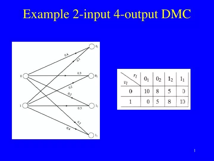
Example 2-input 4-output DMC. Example. Example BSC. Transition probability 0.3’ Recall: MLD decodes to closest codeword in Hamming distance Note: extremely poor channel! Channel capacity = 0.12. Example. 1. 3. 2. 4. 4. 4. 5. 4. 6. 5. 7. 4. 5. 2. 5. 3. 4. 2.

E N D
Example BSC • Transition probability 0.3’ • Recall: MLD decodes to closest codeword in Hamming distance • Note: extremely poor channel! • Channel capacity = 0.12
Example 1 3 2 4 4 4 5 4 6 5 7 4 5 2 5 3 4 2 3 6 6
The Viterbi algorithm for the binary-input AWGN channel • Recall from Chapter 10: • Metrics: Correlation • Decode to the codeword v whose correlation rv with r is maximum • Symbol metrics: rv
Performance bounds • Linear code, and symmetric DMC: • We can w. l. o. g. assume that the all zero codeword is transmitted • ..and that if we make a mistake, the wrong codeword is something else • Thus the decoding mistake will take place at the time instant in the trellis when the wrong codeword and the zero codeword merge • Therefore, interested in the elementary codewords (first event errors)
Performance bounds: BSC • Then the first-event error probability at time t is • Assume that the wrong codeword has weight d Pd: Channel specific
Simplifications of Pd B Pb (E)
Performance bounds: Binary-input AWGN • Asymptotic coding gain = 10 log 10 (Rdfree/2) • BSC derived from AWGN:
Pd for binary-input AWGN v correct: (-1,...,-1) v’ incorrect Sum of d ind.Gaussian random variables (-1,N0/2Es) Count only positions where v’ and v differ
Pd for binary-input AWGN • Asymptotic coding gain = 10 log 10 (Rdfree)
Rate 1/3 convolutional code 3.3 dB • = 10 log10 (1/3*7) = 3.68dB
Some further comments Replace this by a bound • Union bound poor for small SNR • Contributions from higher order terms becomes significant • When to stop the summation? • Other bounds: Divide summation in two parts near/far
Code design: Computer search • Criteria • High dfree • Low Adfree (Low Bdfree)? • High slope/low truncation length* • Use Viterbi algorithm to determine the weight properties • Example:
Example: Viterbi algorithm for distance properties calculation 3 4 6 5 7 6 8 7 5 7 6 7 7 7 7
Suggested exercises • 12.6-12.21