Download
1 / 19
190 likes | 289 Views
Indexes. An index on a file speeds up selections on the search key fields for the index. Any subset of the fields of a relation can be the search key for an index on the relation. Search key is not the same as key (minimal set of fields that uniquely identify a record in a relation).

E N D
Indexes • An index on a file speeds up selections on the search key fields for the index. • Any subset of the fields of a relation can be the search key for an index on the relation. • Search key is not the same as key(minimal set of fields that uniquely identify a record in a relation). • An index contains a collection of data entries, and supports efficient retrieval of all data entries k* with a given key value k.
Alternatives for Data Entry k* in Index • Three alternatives: • Data record with key value k • <k, rid of data record with search key value k> • <k, list of rids of data records with search key k> • Choice of alternative for data entries is orthogonal to the indexing technique used to locate data entries with a given key value k. • Examples of indexing techniques: B+ trees, hash-based structures
Alternatives for Data Entries (2) • Alternative 1: • If this is used, index structure is a file organization for data records (like Heap files or sorted files). • At most one index on a given collection of data records can use Alternative 1. (Otherwise, data records duplicated, leading to redundant storage and potential inconsistency.) • If data records very large, # of pages containing data entries is high. Implies size of auxiliary information in the index is also large, typically.
Alternatives for Data Entries (3) • Alternatives 2 and 3: • Data entries typically much smaller than data records. So, better than Alternative 1 with large data records, especially if search keys are small. • If more than one index is required on a given file, at most one index can use Alternative 1; rest must use Alternatives 2 or 3. • Alternative 3 more compact than Alternative 2, but leads to variable sized data entries even if search keys are of fixed length.
Index Classification • Primary vs. secondary: If search key contains primary key, then called primary index. • Clustered vs. unclustered: If order of data records is the same as, or `close to’, order of data entries, then called clustered index. • Alternative 1 implies clustered, but not vice-versa. • A file can be clustered on at most one search key. • Cost of retrieving data records through index varies greatly based on whether index is clustered or not!
Clustered vs. Unclustered Index Data entries Dataentries (Index File) (Data file) DataRecords Data Records CLUSTERED UNCLUSTERED
Index Classification (Contd.) • Dense vs. Sparse: If there is at least one data entry per search key value (in some data record), then dense. • Alternative 1 always leads to dense index. • Every sparse index is clustered! • Sparse indexes are smaller; Ashby, 25, 3000 22 Basu, 33, 4003 25 Bristow, 30, 2007 30 Ashby 33 Cass, 50, 5004 Cass Smith Daniels, 22, 6003 40 Jones, 40, 6003 44 44 Smith, 44, 3000 50 Tracy, 44, 5004 Sparse Index Dense Index on on Data File Name Age
Index Classification (Contd.) Examples of composite key indexes using lexicographic order. • Composite Search Keys: Search on a combination of fields. • Equality query: Every field value is equal to a constant value. E.g. wrt <sal,age> index: • age=20 and sal =75 • Range query: Some field value is not a constant. E.g.: • age =20; or age=20 and sal > 10 11,80 11 12 12,10 name age sal 12,20 12 13,75 bob 12 10 13 <age, sal> cal 11 80 <age> joe 12 20 10,12 sue 13 75 10 20 20,12 Data records sorted by name 75,13 75 80,11 80 <sal, age> <sal> Data entries in index sorted by <sal,age> Data entries sorted by <sal>
Tree-Based Indexes • ``Find all students with gpa > 3.0’’ • If data is in sorted file, do binary search to find first such student, then scan to find others. • Cost of binary search can be quite high. • Simple idea: Create an `index’ file. Index File kN k2 k1 Data File Page N Page 3 Page 1 Page 2 • Can do binary search on (smaller) index file!
40 51 63 20 33 46* 55* 40* 51* 97* 10* 15* 20* 27* 33* 37* 63* Tree-Based Indexes (2) index entry P K P P K P K m 2 0 1 m 1 2 Root
Index Entries DataEntries B+ Tree: The Most Widely Used Index • Insert/delete at log F N cost; keep tree height-balanced. (F = fanout, N = # leaf pages) • Minimum 50% occupancy (except for root). Each node contains d <= m <= 2d entries. The parameter d is called the order of the tree. Root
Example B+ Tree • Search begins at root, and key comparisons direct it to a leaf. • Search for 5*, 15*, all data entries >= 24* ... 30 24 13 17 39* 22* 24* 27* 38* 3* 5* 19* 20* 29* 33* 34* 2* 7* 14* 16*
B+ Trees in Practice • Typical order: 100. Typical fill-factor: 67%. • average fanout = 133 • Typical capacities: • Height 4: 1334 = 312,900,700 records • Height 3: 1333 = 2,352,637 records • Can often hold top levels in buffer pool: • Level 1 = 1 page = 8 Kbytes • Level 2 = 133 pages = 1 Mbyte • Level 3 = 17,689 pages = 133 MBytes
Inserting a Data Entry into a B+ Tree • Find correct leaf L. • Put data entry onto L. • If L has enough space, done! • Else, must splitL (into L and a new node L2) • Redistribute entries evenly, copy upmiddle key. • Insert index entry pointing to L2 into parent of L. • This can happen recursively • To split index node, redistribute entries evenly, but push upmiddle key. (Contrast with leaf splits.)
Entry to be inserted in parent node. (Note that 17 is pushed up and only 17 this with a leaf split.) 24 30 5 13 Inserting 8* into Example B+ Tree Entry to be inserted in parent node. (Note that 5 is s copied up and • Note: • why minimum occupancy is guaranteed. • Difference between copy-up and push-up. 5 continues to appear in the leaf.) 5* 3* 7* 2* 8* appears once in the index. Contrast
Example B+ Tree After Inserting 8* Root 17 24 30 5 13 39* 2* 3* 19* 20* 22* 24* 27* 38* 5* 7* 8* 29* 33* 34* 14* 16* • Notice that root was split, leading to increase in height. • In this example, we can avoid split by re-distributing entries; however, this is usually not done in practice.
Deleting a Data Entry from a B+ Tree • Start at root, find leaf L where entry belongs. • Remove the entry. • If L is at least half-full, done! • If L has only d-1 entries, • Try to re-distribute, borrowing from sibling (adjacent node with same parent as L). • If re-distribution fails, mergeL and sibling. • If merge occurred, must delete entry (pointing to L or sibling) from parent of L. • Merge could propagate to root, decreasing height.
Example Tree After (Inserting 8*, Then) Deleting 19* and 20* ... • Deleting 19* is easy. • Deleting 20* is done with re-distribution. Notice how middle key is copied up. Root 17 27 30 5 13 39* 2* 3* 22* 24* 27* 29* 38* 5* 7* 8* 33* 34* 14* 16*
... And Then Deleting 24* • Must merge. • Observe `toss’ of index entry (on right), and `pull down’ of index entry (below). 30 39* 22* 27* 38* 29* 33* 34* 5 13 17 30 39* 3* 22* 38* 2* 5* 7* 8* 27* 33* 34* 29* 14* 16*