Download
1 / 20
200 likes | 377 Views
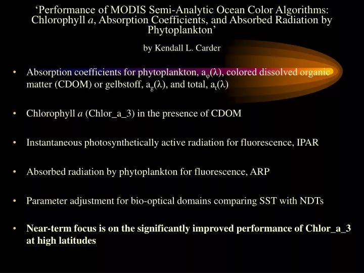
‘Performance of MODIS Semi-Analytic Ocean Color Algorithms: Chlorophyll a , Absorption Coefficients, and Absorbed Radiation by Phytoplankton’ by Kendall L. Carder.

E N D
‘Performance of MODIS Semi-Analytic Ocean Color Algorithms: Chlorophyll a, Absorption Coefficients, and Absorbed Radiation by Phytoplankton’by Kendall L. Carder • Absorption coefficients for phytoplankton, aφ(λ), colored dissolved organic matter (CDOM) or gelbstoff, ag(λ), and total, at(λ) • Chlorophyll a (Chlor_a_3)in the presence of CDOM • Instantaneous photosynthetically active radiation for fluorescence, IPAR • Absorbed radiation by phytoplankton for fluorescence, ARP • Parameter adjustment for bio-optical domains comparing SST with NDTs • Near-term focus is on the significantly improved performance of Chlor_a_3 at high latitudes
a (443)/a(675) versus a (675) from Bering Sea (MF0796) and Antarctic Polar Frontal Zone (REV9802) are compared with high-light tropical and subtropical data (dashed line)
Surface map of (a) Temperature (oC); (b) Nitrate concentration (µM l-1); (c) [chla] (mg m-3); and (d) a (443)/a (675) for the California upwelling region (Cal9704) in April 1997.
Blending scheme to transition between fully packaged and unpackaged pigment parameterization for waters with SST between NDT-1 and NDT+4 degrees C [NDT map from D. Kamekowski]
Performance of new blending scheme for waters of the Southern California Bight transitioning between cold, nutrient-rich upwelled waters and offshore, nutrient-poor waters.
Comparison between Chlor_a_3 SA and OC4v4 algorithms for Chlorophyll a for the Southern California Bight
Chlor_a_3 applied to the Arctic region (a). Quantile plot (b) shows no bias. CZCS algorithm, dashed line in (d), shows bias due to package effect
Chlor_a_3 SA algorithm performance versus OC4v4 for Antarctic based on 971 field data points. Note the large negative bias in the OC4v4 quantile plot
Chlor_a_3 semi-analytical retrievals of chlorophyll a for November 2000
Chlor_a_2 empirical (OC4 surrogate) retrievals of chlorophyll a for November 2000
Semi-analytical retrieval of absorption by CDOM or gelbstoff for November 2000Note the high values in northern (river-rich) hemisphere
Global histograms of chlorophyll a retrievals for November 2000 using a) empirical Chlor_a_2 and b) semi-analytic Chlor_a_3 algorithms. Mean values are 0.215 and 0.325 mg m-3, respectively. Gregg & Conkright (2002)autumn mean = 0.31 mg m-3 .
Match-up Data Sets (preliminary) Provided by the SIMBIOS for Non-Shallow Depths • Chlor_a_3 Chlor_a_2 • Slope: 0.97 0.79 • Intercept: -.0045 -0.012 • r2 0.79 0.79 • Bias 0.009 -0.055 • RMS error 0.173 0.190 • Linear error 49.1% 55.0%
Striping in the Chlor_a_3 products for the western Gulf of Mexico due to stripes in the Lw values: (left) raw and (right) filtered
Raw and filtered data from scene center. Lines 0, 20, 40, … were each averaged horizontally and then averaged together. Similar steps were taken with Lines 1, 21, 41, etc. until a 20-line pattern due to striping was acquired
Noise pattern due to vertical striping from left part of GOM scene (solid). A filter was made by ratioing the mean to each line element and applying to each appropriate line by multiplying. Dashed line is the result. Over-compensation occurred since striping was worse in the lower left than in the upper right portions of original scene.
Change in horizontal variance was about 1% as a result of applying the vertical filter. Note solid and dashed lines represent unfiltered and filtered data.
Conclusions • Chlor_a_3 algorithm performance has improved for high-latitude and upwelling scenes with little or no bias. • SeaWiFS OC-4 algorithm performance in the Southern Ocean for field radiance is biased low by >40%; Chlor_a_2 global mean for November 2000 was 0.215 mg/m3, while Chlor_a_3 value was 0.32 mg/m3. Gregg & Conkright (2002) mean global autumn value was 0.305 mg/m3. • Global ocean primary production calculated with the MODIS Terra Chlor_a_3 algorithm are expected to show an increase over SeaWiFS-based values of about 29% for austral spring data. • Preliminary non-shallow match-up field data for Terra Chlor_a_3 and Chlor_a_2 results show errors of 49% and 55%, respectively, with 1% and –13.5% linear biases, respectively, with most difference occurring for winter California Current data. • A de-striping approach appears promising if smaller sub-scenes are used in the filter generation and application