Download
1 / 24
240 likes | 420 Views
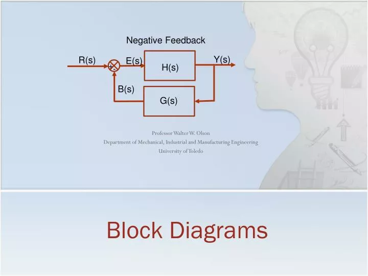
Negative Feedback. Block Diagrams. Y(s). R(s). E(s). H(s). B(s). G(s). Professor Walter W. Olson Department of Mechanical, Industrial and Manufacturing Engineering University of Toledo. +. -. Outline of Today’s Lecture. Review A new way of representing systems

E N D
Negative Feedback Block Diagrams Y(s) R(s) E(s) H(s) B(s) G(s) Professor Walter W. Olson Department of Mechanical, Industrial and Manufacturing Engineering University of Toledo + -
Outline of Today’s Lecture • Review • A new way of representing systems • Coordinate transformation effects • hint: there are none! • Development of the Transfer Function from an ODE • Gain, Poles and Zeros • The Block Diagram • Components • Block Algebra • Loop Analysis • Block Reductions • Caveats
Alternative Method of Analysis • Up to this point in the course, we have been concerned about the structure of the system and discribed that structure with a state space formulation • Now we are going to analyze the system by an alternative method that focuses on the inputs, the outputs and the linkages between system components. • The starting point are the system differential equations or difference equations. • However this method will characterize the process of a system block by its gain, G(s), and the ratio of the block output to its input. • Formally, the transfer function is defined as the ratio of the Laplace transforms of the Input to the Output:
Coordination Transformations • Thus the Transfer function is invariant under coordinate transformation x1 z2 x2 z1
Linear System Transfer Functions General form of linear time invariant (LTI) system is expressed: For an input of u(t)=estsuch that the output is y(t)=y(0)est Note that the transfer function for a simple ODE can be written as the ratio of the coefficients between the left and right sides multiplied by powers of s The order of the system is the highest exponent of s in the denominator.
Gain, Poles and Zeros • The roots of the polynomial in the denominator, a(s), are called the “poles” of the system • The poles are associated with the modes of the system and these are the eigenvalues of the dynamics matrix in a state space representation • The roots of the polynomial in the numerator, b(s) are called the “zeros” of the system • The zeros counteract the effect of a pole at a location • The value of G(s) is the zero frequency or steady state gain of the system
Block Diagrams Actuate Sense Disturbance • Throughout this course, we have used block diagrams to show different properties • Here, we will formalize the meaning of block diagrams Controller u Controller Plant Compute Plant/Process Input r Output y S S kr … State Controller y S S S S Sensor Prefilter D c1 c2 cn-1 cn x … z1 z2 zn zn-1 -K u S State Feedback -1 a1 a2 an-1 an … S S S
Components x The paths represent variable values which are passed within the system xG(s) x Blocks represent System components which are represented by transfer functions and multiply their input signal to produce an output G(s) x+y x Addition and subtraction of signals are represented by a summer block with the operation indicated on the arrow + + y x x Branch points occur when a value is placed on two lines: no modification is made to the signal x
Block Algebra z xGH xGH xGH xH x xG x x G H H GH G + z-x+y x-y x-y z-x+y z-x+y x x y x y z-x x-y + + - - - + + + - - + + + - z x y z y x y
Block Algebra Gx x G(x-z) Gx-z (G-H)x Gx Hx x x x x Gx G-H G G G G G G G H G Gx z Gx-z (G-H)x x x Gx Gx z x + + + + + - - - - - Gx G(x-z) z Gz z G
Block Algebra Gx x x x Gx G G y x-y x x-y x-y x x-y y x x - + + + + + - - - - y y x y G H G H
Closed Loop Systems y r H A positive feedback system + + + - y r H A negative feedback system
Loop Analysis(Very important slide!) Negative Feedback Y(s) R(s) E(s) H(s) B(s) G(s) + -
Loop Analysis Negative Feedback Y(s) R(s) E(s) Positive Feedback H(s) Y(s) R(s) E(s) H(s) B(s) G(s) B(s) + + + -
Block Reduction Example + E y x D C B A First, uncross signals where possible E F y + + + + + + + + + x D C B A - - - - - - G F G
Block Reduction Example + E Next: Reduce Feed Forward Loops where possible y y + + + + + + + + + x x D D C C B B A A - - - - - - - - F F G G
Block Reduction Example y + x Next: Reduce Feedback Loops starting with the inner most + + + + + + D C C B B A - - - - - - y x F F G
Block Reduction Example y x x x y + + + C C B - - - F y
Block Reduction Example x x y y
Loop Nomenclature Disturbance/Noise Reference Input R(s) Error signal E(s) Output y(s) Controller C(s) Plant G(s) Prefilter F(s) Open Loop Signal B(s) Sensor H(s) + + - - The plant is that which is to be controlled with transfer function G(s) The prefilter and the controller define the control laws of the system. The open loop signal is the signal that results from the actions of the prefilter, the controller, the plant and the sensor and has the transfer function F(s)C(s)G(s)H(s) The closed loop signal is the output of the system and has the transfer function
Caveats: Pole Zero Cancellations • Assume there were two systems that were connected as such • An astute student might note thatand then want to cancel the (s+1) term This would be problematic: if the (s+1) represents a true system dynamic, the dynamic would be lost as a result of the cancellation. It would also cause problems for controllability and observability. In actual practice, cancelling a pole with a zero usually leads to problems as small deviations in pole or zero location lead to unpredictable dynamics under the cancellation. Y(s) R(s)
Caveats: Algebraic Loops • The system of block diagrams is based on the presence of differential equation and difference equation • A system built such the output is directly connected to the input of a loop without intervening differential or time difference terms leads to improper block interpretations and an inability to simulate the model. • When this occurs, it is called an Algebraic Loop. Such loops are often meaningless and errors in logic. 2 + -
Summary Negative Feedback • The Block Diagram • Components • Block Algebra • Loop Analysis • Block Reductions • Caveats Y(s) R(s) E(s) x H(s) B(s) G(s) xG(s) x G(s) x+y x + + - + y x x x Next: Bode Plots