Download
1 / 77
780 likes | 1.15k Views
Expectation. Let X denote a discrete random variable with probability function p ( x ) (probability density function f ( x ) if X is continuous ) then the expected value of X, E ( X ) is defined to be:. and if X is continuous with probability density function f ( x ).

E N D
Let X denote a discrete random variable with probability function p(x) (probability density function f(x) if X is continuous) then the expected value of X, E(X) is defined to be: and if X is continuouswith probability density function f(x)
Example: Suppose we are observing a seven game series where the teams are evenly matched and the games are independent. Let X denote the length of the series. Find: • The distribution of X. • the expected value of X, E(X).
Solution: Let A denote theevent that team A, wins and B denote the event that team B wins. Then the sample space for this experiment (together with probabilities and values of X)would be (next slide):
continued • At this stage it is recognized that it might be easier to determine the distribution of X using counting techniques
The possible values of X are {4, 5, 6, 7} • The probability of a sequence of length x is (½)x • The series can either be won by A or B. • If the series is of length x and won by one of the teams (A say) then the number of such series is: • In a series of that lasts x games, the winning team wins 4 games and the losing team wins x - 4 games. The winning team has to win the last games. The no. of ways of choosing the games that the losing team wins is:
Thus The probability of a series of length x. The no. of ways of choosing the winning team • The no. of ways of choosing the games that the losing team wins
Interpretation of E(X) • The expected value of X, E(X), is the centre of gravity of the probability distribution of X. • The expected value of X, E(X), is the long-run average value of X. (shown later –Law of Large Numbers) E(X)
Example: The Binomal distribution Let X be a discrete random variable having the Binomial distribution. i. e. X = the number of successes in n independentrepetitions of a Bernoulli trial. Find the expected value of X, E(X).
Example: A continuous random variable The Exponential distribution Let X have an exponential distribution with parameter l. This will be the case if: • P[X ≥ 0] = 1, and • P[ x ≤ X ≤ x + dx| X ≥ x] = ldx. The probability density function of X is: The expected value of X is:
using integration by parts. We will determine
Summary: If X has an exponential distribution with parameter lthen:
Example: The Uniform distribution Suppose X has a uniform distribution from a to b. Then: The expected value of X is:
Example: The Normal distribution Suppose X has a Normal distribution with parameters mand s. Then: The expected value of X is: Make the substitution:
Hence Now
Example: The Gamma distribution Suppose X has a Gamma distribution with parameters aand l. Then: Note: This is a very useful formula when working with the Gamma distribution.
The expected value of X is: This is now equal to 1.
Thus if X has a Gamma (a ,l) distribution then the expected value of X is: Special Cases: (a ,l) distribution then the expected value of X is: • Exponential (l) distribution:a = 1, l arbitrary • Chi-square (n) distribution:a = n/2, l = ½.
Definition Let X denote a discrete random variable with probability function p(x) (probability density function f(x) if X is continuous) then the expected value of g(X), E[g(X)] is defined to be: and if X is continuouswith probability density function f(x)
Example: The Uniform distribution Suppose X has a uniform distribution from 0to b. Then: Find the expected value of A = X2. If X is the length of a side of a square (chosen at random form 0 to b) then A is the area of the square = 1/3 the maximum area of the square
Example: The Geometric distribution Suppose X (discrete) has a geometric distribution with parameter p. Then: Find the expected value of XA and the expected value of X2.
Recall: The sum of a geometric Series Differentiating both sides with respect to r we get: Differentiating both sides with respect to r we get:
Thus This formula could also be developed by noting:
To compute the expected value of X2. we need to find a formula for Note Differentiating with respect to r we get
implies Thus
Definition Let X be a random variable (discrete or continuous), then the kthmoment of X is defined to be: The first moment of X , m = m1 = E(X) is the center of gravity of the distribution of X. The higher moments give different information regarding the distribution of X.
Definition Let X be a random variable (discrete or continuous), then the kthcentralmoment of X is defined to be: wherem = m1 = E(X) = the first moment of X .
The central moments describe how the probability distribution is distributed about the centre of gravity, m. = 2ndcentral moment. depends on the spread of the probability distribution of X about m. is called the variance of X. and is denoted by the symbolvar(X).
is called the standard deviation of X and is denoted by the symbols. The third central moment contains information about the skewness of a distribution.
The third central moment contains information about the skewness of a distribution. Measure of skewness
The fourth central moment Also contains information about the shape of a distribution. The property of shape that is measured by the fourth central moment is called kurtosis The measure ofkurtosis
Example: The uniform distribution from 0 to 1 Finding the moments