Download

1 / 29
290 likes | 293 Views
Value of Information for Complex Economic Models. Jeremy Oakley Department of Probability and Statistics, University of Sheffield. Paper available from www.sheffield.ac.uk/chebs/papers.html. Outline. Motivation Expected value of perfect information (EVPI)

E N D
Value of Information for Complex Economic Models Jeremy Oakley Department of Probability and Statistics, University of Sheffield. Paper available from www.sheffield.ac.uk/chebs/papers.html
Outline • Motivation • Expected value of perfect information (EVPI) • Emulators and Gaussian processes • Illustration: GERD model
1) Introduction • An economic model is to be used to predict the cost-effectiveness of a particular treatment(s). • The economic model will require the specification of various input parameters. Values of some or all of these are uncertain. • This implies the output of the model, the cost-effectiveness of the treatment is also uncertain.
Introduction • We wish to identify which input parameters are the most influential in driving this output uncertainty. • Should we learn more about these parameters before making a decision?
Introduction • A measure of importance for an input variable have been proposed, based on the expected value of perfect information (EVPI) (Felli and Hazen, 1998, Claxton 1999). • Computing the values of these measures is conventionally done using Monte Carlo techniques. These invariably require a very large numbers of runs of the economic model.
Introduction • For computationally expensive models, this can be completely impractical. • We present an efficient alternative to Monte Carlo, in terms of the number of model runs required.
2) EVPI • We work with net benefit: the monetary value or utility of a treatment is K x efficacy – cost with K the monetary value of a unit increase in efficacy. • The net benefit of any treatment option will be a function of the parameters in the economic model.
EVPI • Denote the net benefit of treatment option t given model parameters X to be NB (t , X ) • Given X, the economic model returns NB (t , X ) for each t . • The ‘true’ values of the model parameters X are uncertain.
EVPI • The baseline decision is to choose t with the largest expected net benefit: NB* = maxt EX{NB (t , X )} • The decision maker will have utility NB*if they choose the best treatment now with no additional information.
EVPI • Now suppose the decision-maker chooses to learn the value of all the uncertain input variables Xbefore choosing a treatment. • They would then choose the treatment with the highest net benefit conditional on X, i.e., they would consider maxt {NB (t , X )}
EVPI • Before actually observing X, they will expect to achieve a net benefit of EX [maxt {NB (t , X )}] • The expected value of this course of action is the expected gain in net benefit over the baseline decision: EX [maxt {NB (t , X )}] – NB*. • This is the (global) EVPI.
Partial EVPI • Now suppose the decision-maker chooses to learn the value of a single uncertain input variable Y , an element of Xbefore making a decision. • They would then choose the treatment with the highest net benefit conditional on Y, i.e., they would consider maxt EX| Y {NB (t , X )}
Partial EVPI • The expected value of learning Y beforeYis actually observed is then: EY[maxt EX|Y {NB (t , X )}] – NB * • This is the partial expected value of perfect information (partial EVPI) for Y. • The partial EVPI is zero if the decision-maker would choose the same treatment for any (plausible) value of Y .
Computing partial EVPIs • We need to evaluate EY[maxt EX|Y {NB (t , X )}] for each element Y in X. • The outer expectation EYis a one-dimensional integral, and can be evaluated using numerical integration. • The term maxt EX|Y is the maximum of (several) higher-dimensional integrals. This requires a large Monte Carlo sample to be evaluated.
Patient Simulation Models • Computing partial EVPIs for computationally cheap models, while not trivial, is relatively straightforward. • However, for one class of models, patient simulation models, a sensitivity analysis using Monte Carlo methods will be out of reach for the model user.
Patient Simulation Models • An example is given in Kanis et al (2002) for modelling osteoporosis: • For an osteoporosis patient, a bone fracture significantly increases the risk of a subsequent fracture. • Residential status of a patient needs to be tracked, in order that costs are not double-counted.
Patient Simulation Models • Progress is to be modelled over a 10 year period. Including the approptiate features in the model necessitates a patient simulation approach. • The net benefit for a given set of input parameters is obtained by sampling events for a large number of patients. • The model takes over an hour for a single run at one set of input parameters.
Patient Simulation Models • For a model with 20 uncertain input variables, computing the partial EVPI reliably using Monte Carlo for each input variable would require a possible minimum of 500,000 model runs. • At one hour for each run, this would take 57 years! • Something more efficient is needed…
3) Emulators • For each treatment option t, and given values for the input parameters X = x, the economic model returns NB (t, x ) • We think of the model as a collection of functions NB (t, x )= ft(x) • Partial EVPIs can be computed more efficiently by exploiting the `smoothness’ of each ft(x)
Emulators • We can compute partial EVPIs more efficiently through the use of an emulator. • An emulator is a statistical model of the original economic model which can then be used as a fast approximation to the model itself. • An approach used by Sacks et al (1989) for dealing with computationally expensive computer models.
Gaussian processes • Any regression technique can be used. We employ a nonparametric regression technique based on Gaussian processes (O’Hagan, 1978). • The gaussian process model for the function ft(x) is non-parametric; the only assumption made about ft(x) is that it is a continuous function.
Gaussian processes • In the Gaussian process model, ft(x) is thought of as an unknown function, and uncertainty about ft(x) is described by a normal distribution. • Correlation between ft(x1) and ft(x2) is modelled parametrically as a function of ||x1-x2||
Gaussian processes • The partial EVPI for input variable Y is given by EY[maxt EX|Y {NB (t , X )}] – NB * • We need to evaluate EX|Y {NB (t , X )} for each t at various values of Y. • Denote G (X |Y) to be the distribution of X given Y. Then EX|Y {NB (t , X )} = ft(x) dG (x |y)
Gaussian processes • We can use Bayesian quadrature (O’Hagan, 1993) to rapidly speed up the computation: • Under the Gaussian process model for ft (x), ft(x) dG (x |y) has a normal distribution, and can be evaluated (almost) instantaneously. • This reduces the number of model runs required from 100,000s to 100s.
4) Example: GERD model • The GERD model, presented in O’Brien et al (1999) predicts the cost-effectiveness of a range of treatment strategies for gastroesophageal reflux disease. • Various uncertain inputs in the model related to treatment efficacies, resource uses by patients. • Model outputs mean number of weeks free of GERD symptoms, and mean cost of treatment for a particular strategy.
Example: GERD model • We consider a choice between three treatment strategies: • Acute treatment with proton pump inhibitors (PPIs) for 8 weeks, then continuous maintenance treatment with PPIs at the same dose. • Acute treatment with PPIs for 8 weeks, then continuous maintenance treatment with hydrogen receptor antagonists (H2RAs). • Acute treatment with PPIs for 8 weeks, then continuous maintenance treatment with PPIs at the a lower dose.
Example: GERD model • There are 23 uncertain input variables. • Distributions for uncertain inputs detailed in Briggs et al (2002). • We estimate the partial EVPI for each input variable, based on 600 runs of the GERD model. • We assume a value of $250 for each week free of GERD symptoms. (It is straightforward to repeat our analysis for alternative values).
Conclusions. • The use of the Gaussian process emulator allows partial EVPIs to be computed considerably more efficiently. • Sensitivity analysis feasible for computationally expensive models. • Can also be extended to value of sample information calculations.