Download
1 / 48
490 likes | 508 Views
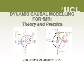
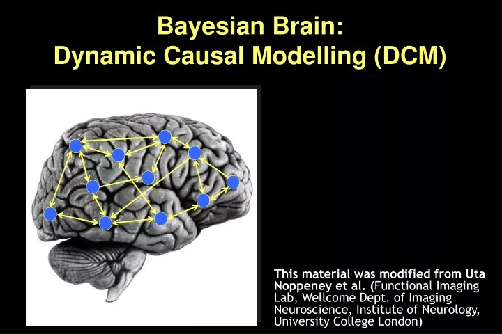
Bayesian Brain: Dynamic Causal Modelling (DCM). This material was modified from Uta Noppeney et al. ( Functional Imaging Lab, Wellcome Dept. of Imaging Neuroscience, Institute of Neurology, University College London). Bounded rationality. Bounded rationality. System 1 Fast

E N D
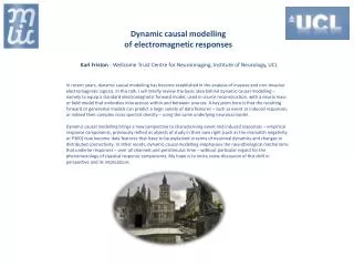
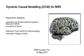
Bayesian Brain: Dynamic Causal Modelling (DCM) This material was modified from Uta Noppeney et al. (Functional Imaging Lab, Wellcome Dept. of Imaging Neuroscience, Institute of Neurology, University College London)
Bounded rationality • System 1 • Fast • Intuitive, associative • heuristics & biases • System 2 • Slow (lazy) • Deliberate, ‘reasoning’ • Rational
Bounded rationality neocortex (system 2) limbic system and brainstem (system 1)
System 1: very prone to biases • Seeing order in randomness • Mental corner cutting • Misinterpretation of incomplete data • Halo effect • False consensus effect • Group think • Self serving bias • Sunk cost fallacy • Cognitive dissonance reduction • Confirmation bias • Authority bias • Small numbers fallacy • In-group bias • Recall bias • Anchoring bias • Inaccurate covariation detection • Distortions due to plausibility
Bounded Rationality • The Small Numbers Problem of Individual Experience • Prone to See Patterns Even in Random Data • Critical Thinking • Decision Supports • Research • Large Ns > individual experience • Controls reduce bias The “Human” Problem Evidence-Based Practice
Evidence-based deciison-making “It’s hard to tell the signal from the noise. The story the data tell us is often the one we’d like to hear, and we usually make sure it has a happy ending. It is when we deny our role in the process that the odds of failure rise.” Nate Silver
전문가들이절대 일어나지 않을 것이라고 주장한 사건 가운데 약 15%가 실제로 일어난다. (전문가들이 반드시 일어날 것이라고 한 사건의 약 25%가 일어나지 않는다.)
스카우팅유망 선수 (베이스볼 아메리카)vs. 각 선수들의 팀 기여도 계산
538 (대통령 선거인단 수)= 435 (하원의원)+ 100 (상원의원)+ 3 (워싱턴 D.C)
당신(아내)이 출장을 마치고 집에 와보니,처음 보는 속옷이 당신 옷장 서랍 속에 들어있다. 나의 배우자(남편)가 날 속이고 바람을 피우고 있을 확률은 얼마나 될까?
사전 확률: 남편이 바람을 피울 확률의 초기 추정치 (P(A)) • 새로운 사건 발생: 수수께끼의 속옷이 발견됐다(P(B)). • 남편이 바람을 피운다는 조건 아래에서 속옷이 등장했을 확률 (P(B|A)) • 사후 확률 당신이 속옷을 발견했다는 조건 아래에서 남편이 바람을 피우고 있을 가능성에 대한 수정된 추정치 (P(A|B))
System analyses in functional neuroimaging Functional specialisation Analyses of regionally specific effects: which areas constitute a neuronal system? Functional integration Analyses of inter-regional effects: what are the interactions between the elements of a given neuronal system? Functional connectivity = the temporal correlation between spatially remote neurophysiological events Effective connectivity = the influence that the elements of a neuronal system exert over another MODEL-free MODEL-dependent
Functional Connectivity • Eigenimage analysis and PCA • Nonlinear PCA • ICA • Effective Connectivity • Psychophysiological Interactions • MAR and State space Models • Structure Equation Models • Volterra Models • Dynamic Causal Models Approaches to functional integration
Psychophysiological interactions Context X source target Set stimuli Context-sensitive connectivity Modulation of stimulus-specific responses source source target target
y y y y y The aim of Dynamic Causal Modeling (DCM) Functional integration and the modulation of specific pathways Contextual inputs Stimulus-free - u2(t) {e.g. cognitive set/time} BA39 Perturbing inputs Stimuli-bound u1(t) {e.g. visual words} STG V4 V1 BA37
Neuronal model Conceptual overview neuronal changes latent connectivity induced connectivity induced response Input u(t) The bilinear model c1 b23 neuronal states a12 activity z2(t) activity z3(t) Neural activity z1(t) y Hemodynamic model y y BOLD
Likelihood Prior probability Posterior probability Rational statistical inference(Bayes, Laplace) Sum over space of hypotheses
Conceptual overview • Models of • Responses in a single region • Neuronal interactions • Constraints on • Connections • Biophysical parameters Bayesian estimation posterior likelihood ∙ prior
LG left FG right LG right FG left Example: linear dynamic system LG = lingual gyrus FG = fusiform gyrus Visual input in the - left (LVF) - right (RVF)visual field. z4 z3 z1 z2 RVF LVF u2 u1 systemstate input parameters state changes effective connectivity externalinputs
LG left FG right LG right FG left Extension: bilinear dynamic system z4 z3 z1 z2 CONTEXT RVF LVF u2 u3 u1
Bilinear state equation in DCM modulation of connectivity systemstate direct inputs state changes intrinsic connectivity m externalinputs
Neuronal model Conceptual overview neuronal changes latent connectivity induced connectivity induced response Input u(t) The bilinear model c1 b23 neuronal states a12 activity z2(t) activity z3(t) activity z1(t) y y y Hemodynamic model BOLD
The hemodynamic “Balloon” model • 5 hemodynamic parameters: important for model fitting, but of no interest for statistical inference • Empirically determinedprior distributions. • Computed separately for each area (like the neural parameters).
ηθ|y stimulus function u Overview:parameter estimation neural state equation • Combining the neural and hemodynamic states gives the complete forward model. • An observation model includes measurement errore and confounds X (e.g. drift). • Bayesian parameter estimationby means of a Levenberg-Marquardt gradient ascent, embedded into an EM algorithm. • Result:Gaussian a posteriori parameter distributions, characterised by mean ηθ|y and covariance Cθ|y. parameters hidden states state equation observation model modelled BOLD response
Overview:parameter estimation • Models of • Responses in a single region • Neuronal interactions • Constraints on • Connections • Biophysical parameters posterior likelihood ∙ prior Bayesian estimation
needed for Bayesian estimation, embody constraints on parameter estimation express our prior knowledge or “belief” about parameters of the model hemodynamic parameters:empirical priors temporal scaling:principled prior coupling parameters:shrinkage priors Priors in DCM Bayes Theorem posterior likelihood ∙ prior
Shrinkage priorsfor coupling parameters (η=0)→ conservative estimates! Priors in DCM • Principled priors: • System stability:in the absence of input, the neuronal states must return to a stable mode • Constraints on prior variance of intrinsic connections (A): Probability <0.001 of obtaining a non-negative Lyapunov exponent (largest real eigenvalue of the intrinsic coupling matrix) • Self-inhibition: Priors on the decay rate constant σ (ησ=1, Cσ=0.105); these allow for neural transients with a half life in the range of 300 ms to 2 seconds • Temporal scaling: Identical in all areas by factorising A and B with σ (a single rate constant for all regions): all connection strengths are relative to the self-connections.
Shrinkage Priors Small & variable effect Large & variable effect Small but clear effect Large & clear effect
EM and gradient ascent • Bayesian parameter estimation by means of expectation maximisation (EM) • E-step:gradient ascent (Fisher scoring & Levenberg-Marquardt regularisation) to compute • (i) the conditional mean ηθ|y(= expansion point of gradient ascent), • (ii) the conditional covariance Cθ|y • M-step:Estimation of hyperparameters ifor error covariance components Qi: • Note: Gaussian assumptions about the posterior (Laplace approximation)
ηθ|y Parameter estimation in DCM • Bayesian parameter estimation under Gaussian assumptions by means of EM and gradient ascent. • Result:Gaussian a posteriori parameter distributions with mean ηθ|y and covariance Cθ|y. • Combining the neural and hemodynamic states gives the complete forward model: • The observation model includes measurement error and confounds X (e.g. drift):
Hypothesis abouta neural system The DCM cycle Statistical test on parameters of optimal model Definition of DCMs as systemmodels Bayesian modelselection of optimal DCM Design a study thatallows to investigatethat system Parameter estimationfor all DCMs considered Data acquisition Extraction of time seriesfrom SPMs
Planning a DCM-compatible study • Suitable experimental design: • preferably multi-factorial (e.g. 2 x 2) • e.g. one factor that varies the driving (sensory) input • and one factor that varies the contextual input • Hypothesis and model: • define specific a priori hypothesis • Which alternative models? • which parameters are relevant to test this hypothesis? • TR: • as short as possible (optimal: < 2 s)