Download
1 / 46
490 likes | 526 Views
An Introduction to Clustering. Qiang Yang Adapted from Tan et al. and Han et al. Clustering Definition. Given a set of data points, each having a set of attributes, and a similarity measure among them, Find clusters such that Data points in one cluster are more similar to one another.

E N D
An Introduction to Clustering Qiang Yang Adapted from Tan et al. and Han et al.
Clustering Definition • Given a set of data points, • each having a set of attributes, and • a similarity measure among them, • Find clusters such that • Data points in one cluster are more similar to one another. • Data points in separate clusters are less similar to one another. • Similarity Measures: • Euclidean distance if attributes are continuous. • Other problem-specific measures.
Illustrating Clustering • Euclidean Distance Based Clustering in 3-D space. Intra-cluster distance is minimized Inter-cluster distance is maximized
Clustering: Application 1 • Market Segmentation: • Goal: divide a market into distinct subsets of customers where any subset may conceivably be selected as a market target to be reached with a distinct marketing mix. • Approach: • Collect different attributes of customers based on their geographical and lifestyle related information. • Find clusters of similar customers. • Measure the clustering quality by observing buying patterns of customers in same cluster vs. those from different clusters.
Clustering: Application 2 • Document Clustering: • Goal: To find groups of documents that are similar to each other based on the important terms appearing in them. • Approach: • To identify frequently occurring terms in each document. • Form a similarity measure based on the frequencies of different terms. • Use it to cluster. • Information Retrieval can utilize the clusters to relate a new document or search term to clustered documents.
Illustrating Document Clustering • Clustering Points: 3204 Articles of Los Angeles Times. • Similarity Measure: How many words are common in these documents (after some word filtering).
Clustering of S&P 500 Stock Data • Observe Stock Movements every day. • Clustering points: Stock-{UP/DOWN} • Similarity Measure: Two points are more similar if the events described by them frequently happen together on the same day. • We used association rules to quantify a similarity measure.
Distance Measures Tan et al. From Chapter 2
Similarity and Dissimilarity • Similarity • Numerical measure of how alike two data objects are. • Is higher when objects are more alike. • Often falls in the range [0,1] • Dissimilarity • Numerical measure of how different are two data objects • Lower when objects are more alike • Minimum dissimilarity is often 0 • Upper limit varies • Proximity refers to a similarity or dissimilarity
Euclidean Distance • Euclidean Distance Where n is the number of dimensions (attributes) and pk and qk are, respectively, the kth attributes (components) or data objects p and q. • Standardization is necessary, if scales differ.
Euclidean Distance Distance Matrix
Minkowski Distance • Minkowski Distance is a generalization of Euclidean Distance Where r is a parameter, n is the number of dimensions (attributes) and pk and qk are, respectively, the kth attributes (components) or data objects p and q.
Minkowski Distance: Examples • r = 1. City block (Manhattan, taxicab, L1 norm) distance. • A common example of this is the Hamming distance, which is just the number of bits that are different between two binary vectors • r = 2. Euclidean distance • r. “supremum” (Lmax norm, Lnorm) distance. • This is the maximum difference between any component of the vectors • Example: L_infinity of (1, 0, 2) and (6, 0, 3) = ?? • Do not confuse r with n, i.e., all these distances are defined for all numbers of dimensions.
Minkowski Distance Distance Matrix
Mahalanobis Distance is the covariance matrix of the input data X B When the covariance matrix is identity Matrix, the mahalanobis distance is the same as the Euclidean distance. Useful for detecting outliers. Q: what is the shape of data when covariance matrix is identity?Q: A is closer to P or B? A P For red points, the Euclidean distance is 14.7, Mahalanobis distance is 6.
Mahalanobis Distance Covariance Matrix: C A: (0.5, 0.5) B: (0, 1) C: (1.5, 1.5) Mahal(A,B) = 5 Mahal(A,C) = 4 B A
Common Properties of a Distance • Distances, such as the Euclidean distance, have some well known properties. • d(p, q) 0 for all p and q and d(p, q) = 0 only if p= q. (Positive definiteness) • d(p, q) = d(q, p) for all p and q. (Symmetry) • d(p, r) d(p, q) + d(q, r) for all points p, q, and r. (Triangle Inequality) where d(p, q) is the distance (dissimilarity) between points (data objects), p and q. • A distance that satisfies these properties is a metric, and a space is called a metric space
Common Properties of a Similarity • Similarities, also have some well known properties. • s(p, q) = 1 (or maximum similarity) only if p= q. • s(p, q) = s(q, p) for all p and q. (Symmetry) where s(p, q) is the similarity between points (data objects), p and q.
Similarity Between Binary Vectors • Common situation is that objects, p and q, have only binary attributes • Compute similarities using the following quantities M01= the number of attributes where p was 0 and q was 1 M10 = the number of attributes where p was 1 and q was 0 M00= the number of attributes where p was 0 and q was 0 M11= the number of attributes where p was 1 and q was 1 • Simple Matching and Jaccard Distance/Coefficients SMC = number of matches / number of attributes = (M11 + M00) / (M01 + M10 + M11 + M00) J = number of value-1-to-value-1 matches / number of not-both-zero attributes values = (M11) / (M01 + M10 + M11)
SMC versus Jaccard: Example p = 1 0 0 0 0 0 0 0 0 0 q = 0 0 0 0 0 0 1 0 0 1 M01= 2 (the number of attributes where p was 0 and q was 1) M10= 1 (the number of attributes where p was 1 and q was 0) M00= 7 (the number of attributes where p was 0 and q was 0) M11= 0 (the number of attributes where p was 1 and q was 1) SMC = (M11 + M00)/(M01 + M10 + M11 + M00) = (0+7) / (2+1+0+7) = 0.7 J = (M11) / (M01 + M10 + M11) = 0 / (2 + 1 + 0) = 0
Cosine Similarity • If d1 and d2 are two document vectors, then cos( d1, d2 ) = (d1d2) / ||d1|| ||d2|| , where indicates vector dot product and || d || is the length of vector d. • Example: d1= 3 2 0 5 0 0 0 2 0 0 d2 = 1 0 0 0 0 0 0 1 0 2 d1d2= 3*1 + 2*0 + 0*0 + 5*0 + 0*0 + 0*0 + 0*0 + 2*1 + 0*0 + 0*2 = 5 ||d1|| = (3*3+2*2+0*0+5*5+0*0+0*0+0*0+2*2+0*0+0*0)0.5 = (42) 0.5 = 6.481 ||d2|| = (1*1+0*0+0*0+0*0+0*0+0*0+0*0+1*1+0*0+2*2)0.5= (6) 0.5 = 2.245 cos( d1, d2 ) = .3150, distance=1-cos(d1,d2)
Clustering: Basic Concepts Tan et al. Han et al.
The K-Means Clustering Method: for numerical attributes • Given k, the k-means algorithm is implemented in four steps: • Partition objects into k non-empty subsets • Compute seed points as the centroids of the clusters of the current partition (the centroid is the center, i.e., mean point, of the cluster) • Assign each object to the cluster with the nearest seed point • Go back to Step 2, stop when no more new assignment
The mean point can be influenced by an outlier The mean point can be a virtual point
10 9 8 7 6 5 4 3 2 1 0 0 1 2 3 4 5 6 7 8 9 10 The K-Means Clustering Method • Example 10 9 8 7 6 5 Update the cluster means Assign each objects to most similar center 4 3 2 1 0 0 1 2 3 4 5 6 7 8 9 10 reassign reassign K=2 Arbitrarily choose K object as initial cluster center Update the cluster means
Optimal Clustering Sub-optimal Clustering K-means Clusterings Original Points
10 9 8 7 6 5 4 3 2 1 0 0 1 2 3 4 5 6 7 8 9 10 10 9 8 7 6 5 4 3 2 1 0 0 1 2 3 4 5 6 7 8 9 10 What is the problem of k-Means Method? • The k-means algorithm is sensitive to outliers ! • Since an object with an extremely large value may substantially distort the distribution of the data. • K-Medoids: Instead of taking the mean value of the object in a cluster as a reference point, medoids can be used, which is the most centrally located object in a cluster.
The K-MedoidsClustering Method • Find representative objects, called medoids, in clusters • Medoids are located in the center of the clusters. • Given data points, how to find the medoid? 10 9 8 7 6 5 4 3 2 1 0 0 1 2 3 4 5 6 7 8 9 10
Categorical Values • Handling categorical data: k-modes (Huang’98) • Replacing means of clusters with modes • Mode of an attribute: most frequent value • Mode of instances: for an attribute A, mode(A)= most frequent value • K-mode is equivalent to K-means • Using a frequency-based method to update modes of clusters • A mixture of categorical and numerical data: k-prototype method
Density-Based Clustering Methods • Clustering based on density (local cluster criterion), such as density-connected points • Major features: • Discover clusters of arbitrary shape • Handle noise • One scan • Need density parameters as termination condition • Several interesting studies: • DBSCAN: Ester, et al. (KDD’96) • OPTICS: Ankerst, et al (SIGMOD’99). • DENCLUE: Hinneburg & D. Keim (KDD’98) • CLIQUE: Agrawal, et al. (SIGMOD’98)
Density-Based Clustering • Clustering based on density (local cluster criterion), such as density-connected points • Each cluster has a considerable higher density of points than outside of the cluster
p MinPts = 5 e = 1 cm q Density-Based Clustering: Background • Two parameters: • e: Maximum radius of the neighbourhood • MinPts: Minimum number of points in an Eps-neighbourhood of that point • Ne(p): {q belongs to D | dist(p,q) <= e} • Directly density-reachable: A point p is directly density-reachable from a point q wrt. e, MinPts if • 1) p belongs to Ne(q) • 2) core point condition: |Ne (q)| >= MinPts
DBSCAN: Core, Border and Noise Points Original Points Point types: core, border and noise Eps = 10, MinPts = 4
p q o Density-Based Clustering • Density-reachable: • A point p is density-reachable from a point q wrt. e, MinPts if there is a chain of points p1, …, pn, p1 = q, pn = p such that pi+1 is directly density-reachable from pi • Density-connected • A point p is density-connected to a point q wrt. e, MinPts if there is a point o such that both, p and q are density-reachable from o wrt. e and MinPts. p p1 q
Outlier Border Eps = 1cm MinPts = 5 Core DBSCAN: Density Based Spatial Clustering of Applications with Noise • Relies on a density-based notion of cluster: A cluster is defined as a maximal set of density-connected points • Discovers clusters of arbitrary shape in spatial databases with noise
DBSCAN Algorithm • Eliminate noise points • Perform clustering on the remaining points
DBSCAN Properties • Generally takes O(nlogn) time • Still requires user to supply Minpts and e • Advantage • Can find points of arbitrary shape • Requires only a minimal (2) of the parameters
Clusters When DBSCAN Works Well Original Points • Resistant to Noise • Can handle clusters of different shapes and sizes
DBSCAN: Determining EPS and MinPts • Idea is that for points in a cluster, their kth nearest neighbors are at roughly the same distance • Noise points have the kth nearest neighbor at farther distance • So, plot sorted distance of every point to its kth nearest neighbor
Using Similarity Matrix for Cluster Validation • Order the similarity matrix with respect to cluster labels and inspect visually.
Using Similarity Matrix for Cluster Validation • Clusters in random data are not so crisp DBSCAN
Using Similarity Matrix for Cluster Validation • Clusters in random data are not so crisp K-means