Download
1 / 33
340 likes | 589 Views
Full Wave Simulation and Validation of a Simple Via Structure. Bruce Archambeault , Samuel Connor, Daniel N. de Araujo, C. Schuster, A.Ruehli, IBM barch@us.ibm.com , sconnor@us.ibm.com , dearaujo@us.ibm.com , cschuste@us.ibm.com , ruehli@us.ibm.com

E N D
Full Wave Simulation and Validation of a Simple Via Structure Bruce Archambeault, Samuel Connor, Daniel N. de Araujo, C. Schuster, A.Ruehli, IBM barch@us.ibm.com, sconnor@us.ibm.com, dearaujo@us.ibm.com, cschuste@us.ibm.com, ruehli@us.ibm.com M. R. Has hemi, R. Mistral, Pennsylvania State University mmh244 @engr.psu.edu, mittra@engr.psu.edu
PCBs and Very High Frequency Data Rates • Gaga-bit signal rates in common practice today • 10-12 Gb/s plan in near future • Require at least 5th harmonic for reasonable signal quality • 12 Gb/s 30 GHz • Both measurements and simulations require extreme care at these frequencies!
Measurements @ 10-50 GHz+ • Calibration of VNA requires special calibration fixtures • Special probing techniques • Extremely expensive equipment • Requires costly PCBs with various structures to be studied • Difficult but possible
Full Wave Electromagnetic Simulations • Can save costs associated with test equipment and test PCBs • Eliminate calibration concerns • Probes within models can be ‘perfect’ • No impact on results from the act of measuring • Software tools are mature and reasonably priced (sometimes)
Many layers Entry/exit on different layers Inexpensive dielectrics have more loss at high frequencies Need to be able to properly analyze all effects Quasi-static models not accurate at high frequencies The High Speed PCB Problem
Source 100 mil 10 mil 10 mil 50 mil Round Geometries! Load Initial GeometrySingle Plane for Initial Models Dielectric Constant = 3.8 Trace Thickness = 1 mil Via Barrel Diameter = 20 mil Plane thickness = 1 mil Via Antipad Diameter = 44 mil Trace terminated in characteristic impedance = 80 Ohm Via Pad Diameter = 34 mil PCB size = 300 mil x 300 mil Trace width = 7 mil Metal = perfect electric conductor Loss tan = 0 Absorbing boundary conditions! Background DC = 1
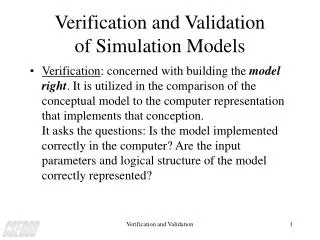
Validation of Simulation Results Extremely Important • Measurement data not available • Assumptions must be known • By user • Built into the software • Inherent in simulation technique • Different techniques have different assumptions! • Simulation validation by using multiple modeling techniques
How Good is “Good”? • “I know it when I see it” • Feature Selective Validation (FSV) technique • Allows a numerical comparison that agrees with ‘experts’ • Used in IEEE Standard on Model Validation • Performs an FFT, separates low frequency data and high frequency data • Low frequency data provides indication of overall amplitude agreement (ADM) • High frequency data provides indication of rapidly changing feature agreement (FDM)
FSV Results for ADMExample (One Plot for Each Pair of Techniques) cFDTD vs FIT PEEC vs FDTD
FSV Grade and Spread • Easier to quickly compare plots • Grade Number of categories required to get 85% Confidence starting at highest (excellent agreement) • Quality of agreement • Spread Number of categories required to get 85% Confidence starting with the largest category • Consistency of the agreement
Techniques Grade Spread cFDTD-FIT 2 2 cFDTD-FDTD 4 4 cFDTD-FEM 1 1 cFDTD-PEEC 3 3 FIT-FDTD 4 4 FIT-FEM 2 2 FIT-PEEC 3 3 FTDT-FEM 5 4 FDTD-PEEC 4 4 FEM-PEEC 3 3 Average 3.1 (Excellent-Good) 3.0 (Excellent-Good) Summary of FSV Grade/Spread for Initial Agreement Between Techniques
Grade Spread FDTD-CST 4 4 FDTD-PEEC 3 3 CST-PEEC 3 3 FSV Results Excellent-to-Very Good FDTD-PEEC FDTD-FIT PEEC-FIT
Traces often Enter/Exit in different DirectionsWill This Make a Difference? Zero Degrees between entry/exit traces 90 Degrees between entry/exit traces 180 Degrees between entry/exit traces
Two Plane Geometry Dielectric Constant = 3.8 Trace Thickness = 1 mil Via Barrel Diameter = 20 mil Plane thickness = 1 mil Via Antipad Diameter = 44 mil Trace terminated in characteristic impedance = 80 Ohm Via Pad Diameter = 34 mil PCB size = 300 mil x 300 mil Trace width = 7 mil Metal = perfect electric conductor Loss tan = 0 Absorbing boundary conditions! Background DC = 1
Grade Spread FDTD-MWS 3 3 FDTD-HFSS 3 3 MWS-HFSS 3 3 Validation Using Different Techniques
Real-World PCBs have many Layers/Planes 6 Plane Example 10 Plane Example
Model Detail Subtleties • Assumptions may be hidden • Simulation techniques • Software simulation tool • User
Model Detail Subtleties Examples • Dielectric slab vs background dielectric • Volume based techniques can handle dielectric slabs without significant increase in computer resources • FDTD, FIT, FEM • Surface based techniques require significant increase in computer resources for dielectric slab • Background dielectric easy to simulate • MoM, PEEC • Does it matter?
Model Detail Subtleties Examples • Round vs Square objects • Via, Via pad, Via antipad • Some techniques have non-rectangular grids to make closer approximation to round objects • FEM • Some software tools handle round objects with special internal calculations • ‘Regular’ rectangular grids require stairstepping for round objects • Does it matter?
Models Can Provide Information that is Impossible to Measure • Examples • Current through ground return via • Displacement return current mapping
Ground-Return Via Current from FDTD Simulation (Time Domain)
Ground-Return Via Current from FDTD Simulation (Frequency Domain)
View of Displacement Current Through Dielectric(Two Ground-Return Vias)
Summary • Model validation is IMPORTANT • Do NOT simply believe simulation results because a technique or tool was accurate on a different model!!! • FSV technique allows user to compare overall quality of agreement • Similar to expert opinion • Modeling allows the user to view voltage/currents/fields in ways not possible in the laboratory • Helps understand underlying physics • Helps with validation • Via configuration changes transmission at high frequencies significantly
FSV Follow up • FSV Web site • http://www.eng.dmu.ac.uk/~apd/FSV/FSV%20web/ • On-line Survey • http://orlandi.ing.univaq.it/test/default.asp • FSV Program free download • http://ing.univaq.it/uaqemc/public_html/