Download
1 / 12
120 likes | 211 Views
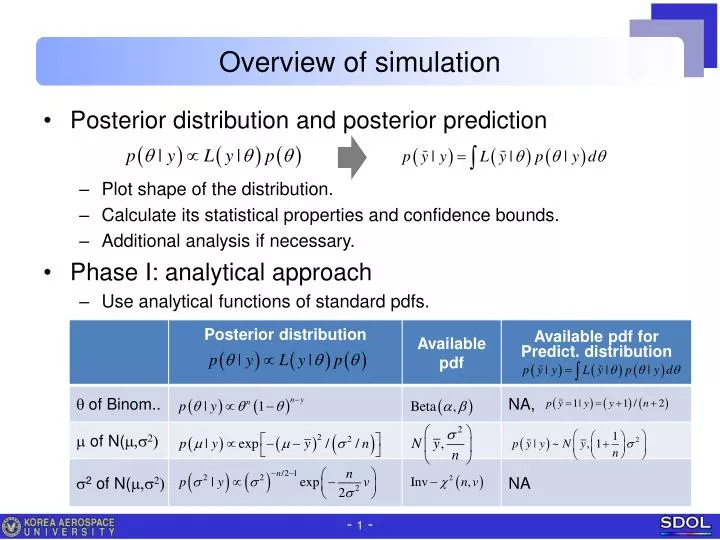
Overview of simulation. Posterior distribution and posterior prediction Plot shape of the distribution. Calculate its statistical properties and confidence bounds. Additional analysis if necessary. Phase I: analytical approach Use analytical functions of standard pdfs . .

E N D
Overview of simulation • Posterior distribution and posterior prediction • Plot shape of the distribution. • Calculate its statistical properties and confidence bounds. • Additional analysis if necessary. • Phase I: analytical approach • Use analytical functions of standard pdfs.
Overview of simulation • Phase II: sampling approach based on factorization • Use sampling technique of standard pdfs. • Draw s2 from the marginal pdf • Draw m from the conditional pdf
Overview of simulation • Phase III: sampling approach based on factorization • Use sampling technique of inverse CDF for general case. • Draw a from the marginal pdf p(a|y) . • Draw b from the conditional pdf p(b|a,y).
Overview of simulation • Remark • For more complicated & practical problems, analytic treatment of posterior distribution become more and more difficult or impossible. • A battery of powerful methods has been developed over the past few decades for simulating from probability distributions. • References • Chap10 & 11 of Gelman • Andrieu, C., et al. (2003). An Introduction to MCMC for Machine Learning. Machine Learning, 50, 5–43. • Methods of simulation • Grid method (inverse CDF method) • Rejection sampling • Importance sampling • Markov Chain Monte Carlo (MCMC) method
Grid method (inverse CDF method) • Procedure • In order to generate samples following pdf f(v), • Construct approx. cdf F(v) which is the integral of f(v). • Draw random value U from the uniform distribution on [0,1]. • let v=F-1(U). Then the value v will be a random draw from f(v). • Practice with matlab • Remarks • Effective only when we have knowledge of the range and we miss nothing outside their ranges. • Not good for higher-dimensional multivariate problems, where computing at every point in the multidimensional grid becomes prohibitively expensive. • Conclusion: this method is not used well in practice.
Rejection sampling • Procedure • In order to generate samples for pdf p(x), introduce an arbitrary pdf q(x) that has sampling capability, such that Mq(x) covers whole p(x). • Sample q at random from the proposal pdf q(x). • With probability p(x)/(Mq(x)), accept x as a draw from p. • M is just chosen such that Mq exceeds p at everywhere. • Pseudo-code & illustration
Rejection sampling • Practice with matlab • generate samples of this distribution. • Remarks • it is not always possible to bound p/q with reasonable amount M over the whole space. If M is too large, the acceptance probability Pr(x accepted) ~ 1/M is too small.
Importance sampling • Calculation of moment • Introduce an arbitrary pdf q(x) that has sampling capability. In this case, q(x) need not cover p(x). • Then moment (or expectation) of an arbitrary function f(x) becomes • In case p(x) is not normalized, normalize the weight samples. • Practice with matlab • Calculate mean & variance of p(x) using importance sampling. where x(i) is the sample drawn from q(x).
Importance sampling • Calculation of probability • In case that we can draw samples from p(x) This is to count # of x where g<0, or sum all Ig where Ig is 1 when g<0. • In case that we can’t draw samples, This is to sum all Ig but with uneven weight where Ig is 1 when g<0. • Practice with matlab • Calculate P[p(x)<5] using importance sampling. where Ig is 1 when g(x)<0.
Importance sampling • Generation of samples • Recall that • Another meaning of this is that the distribution p(x) has weight w(xi) at the sample points xidrawn by q(x). This can be written as • Practice with matlab • Generate samples of this distribution.
General guidelines • From Chap10 of Gelman • Use of simulation in the Bayesian analysis • Inferences are conveniently conducted using random sampling from the posterior distribution, which include percentiles at 2.5%, 25%, …. • Once simulations obtained, it is also easy to draw samples for predictive distribution. For each draw of q from p(q|y), just draw one ͠yfrom p(͠y|q). • Normalized vsunnormalized distribution • We assume that the target density p(q|y), being a function of q, can be easily computed for any value of q whether it is closed form or not. • We assume that the density need not be normalized, it is just OK if it is proportional to the true distribution. • Crude or first hand estimation • Rough estimate of the location of the distribution – that is, a point estimate of the parameters - using some simple technique is necessary. • Finding modes by optimization or Newton’s method may also be needed.
General guidelines • How many simulation draws needed ?