Download
1 / 21
260 likes | 355 Views
Mathematical Modeling in Biology:. incorporating mathematical biology in lower-level math courses. Glenn Ledder Department of Mathematics University of Nebraska-Lincoln gledder@math.unl.edu. Overview. Mathematical modeling Curve fitting, simulation, and modeling

E N D
Mathematical Modeling in Biology: incorporating mathematical biology in lower-level math courses Glenn Ledder Department of Mathematics University of Nebraska-Lincoln gledder@math.unl.edu
Overview • Mathematical modeling • Curve fitting, simulation, and modeling • Models in biology vs models in physics • Modeling by discovery • Examples • Structured populations • Pharmacokinetics • Predator-prey dynamics • Resource management
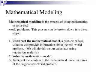
Mathematical Models A mathematical model is a well-defined mathematical object consisting of a collection of variables and rules governing their values. Models are created from assumptions inspired by observation of some real phenomena in the hope that the model behavior resembles the real behavior.
Curve Fitting and Simulation • Using data to obtain parameter values is curve fitting, not modeling. • There is an underlying model in parameter determination, but the model is assumed. • Using a computer to predict the behavior of some real scenario is simulation, not modeling. • Simulation involves computation with an assumed model.
Mathematical Modeling • Mathematical modeling is the process of constructing, testing, and improving mathematical models. • Mathematical models should be general in the sense of containing parameters that can be adjusted to strengthen, weaken, or modify the behavior of each process. • They do not need to be general in the sense of working for all possible cases.
Models in Biology and Physics • Most physical processes are well described by “physical laws” valid in a wide variety of settings. • It is easy to get physical science models right. • Most biological processes are too complicated to be described by simple mathematical formulas. • It is hard to get good models for biology. • A model that works in one setting may fail in a different setting.
Modeling by Discovery • Mathematical modeling requires good scientific intuition. • Scientific intuition can be developed by observation. • Detailed observation in biological scenarios can be very difficult or very time-consuming, so can seldom be done in a math course.
Presenting “bugbox”, a simple computer simulation for structured population dynamics! Because bugbox is a simulation, its behavior doesn’t necessarily match any real insect population. It functions as a biology lab for a virtual world. The front-end for bugbox is not quite finished. Eventually, it will run as a maplet on a server at the UNL Math Department.
Structured Population Dynamics The final “bugbox” model: Let Lt be the number of larvae at time t. Let Jt be the number of juveniles at time t. Let At be the number of adults at time t. Lt+1 = sLLt+fAt Jt+1 = sJJt+pLLt At+1 = sAAt+pJJt
Things to do with the model: • Write as xt+1 = Mxt. • Run a simulation to see that x evolves to a fixed ratio independent of initial conditions. • Obtain the problem Mxt= λxt. • Develop eigenvalues and eigenvectors. • Show that the term with largest |λ| dominates and note that the largest eigenvalue is always positive. • Note the significance of the largest eigenvalue. • Use it to predict long-term behavior and discuss its shortcomings.
Pharmacokinetics x′ = Q(t) – (k1+r) x + k2y y′ = k1x – k2y Q(t) k1x blood tissues k2y x(t) y(t) rx
Predator-Prey Dynamics • Lotka-Volterra x = prey, y = predator x′ = rx–sxy y′ = esxy – my Predicts oscillations of varying amplitude
Predator-Prey Dynamics • Lotka-Volterra x = prey, y = predator x′ = rx–sxy y′ = esxy – my Predicts oscillations of varying amplitude Predicts impossibility of predator extinction.
Predator-Prey Dynamics • logistic x = prey, y = predator x′ = rx(1 – — )– sxy y′ = esxy – my Predicts stable xy equilibrium if mis small enough x K
Predator-Prey Dynamics • logistic x = prey, y = predator x′ = rx(1 – — )– sxy y′ = esxy – my Predicts stable xy equilibrium if mis small enough and y→0 if m too large x K
Predator-Prey Dynamics • Holling type 2 x = prey, y = predator x′ = rx(1 – — )– —––– y′ = —––– – my x K sxy 1 + Hx esxy 1 + Hx
sxy 1 + Hx Why —–––? Let s be search rate Let P be predation rate per predator Let f be fraction of time spent searching Let h be the time needed to handle one prey P=fsxand f + hP =1 P =—–––– sx 1 + shx
Predator-Prey Dynamics • Holling type 2 x = prey, y = predator x′ = rx(1 – — )– —––– y′ = —––– – my Predicts stable xy equilibrium if mis small enough. x K sxy 1 + Hx esxy 1 + Hx
Predator-Prey Dynamics • Holling type 2 x = prey, y = predator x′ = rx(1 – — )– —––– y′ = —––– – my Predicts stable xy equilibrium if mis small enough and stable limit cycle if m iseven smaller. x K sxy 1 + Hx esxy 1 + Hx
Resource Management • Holling type 3 x = resource, y = consumer x′ = rx(1 – — )– —–––– y′ = —–––– – my Now assume y is a parameter. x K sx2y 1 + Hx2 esx2y 1 + Hx2 x′ = rx(1 – — )– —–––– cx2 1 + Hx2 x K
x′ = rx(1 – — )– —–––– cx2 1 + Hx2 x K Things to do with the model: • Nondimensionalize it. CX2 A + X2 X′ = X (1 – X) – —––– • Find equilibrium solutions graphically. • Create a bifurcation diagram for given A. • Choose C to optimize yield [X(1–X)]