Download

1 / 15
270 likes | 871 Views
Practical Data Science with R - Choosing and evaluating models. Kim Jeong Rae UOS.DML. 2014.11.3. Contents. Mapping problems to machine learning tasks Evaluating models Evaluating classification models Evaluating scoring models Evaluating probability models Evaluating ranking models

E N D
Practical Data Sciencewith R- Choosing and evaluating models Kim Jeong Rae UOS.DML. 2014.11.3.
Contents • Mapping problems to machine learning tasks • Evaluating models • Evaluating classification models • Evaluating scoring models • Evaluating probability models • Evaluating ranking models • Evaluating clustering models • Validating models
Mapping problems to machine learning tasks Some common Classification method
Evaluating models – classification models(1/2) spamD <- read.table('spamD.tsv',header=T,sep='\t') spamTrain <- subset(spamD,spamD$rgroup>=10) # Spliting Test/Train data spamTest <- subset(spamD,spamD$rgroup<10) # Spliting Test/Train data spamVars <- setdiff(colnames(spamD),list('rgroup','spam')) # Deleting selection columns spamFormula <- as.formula(paste('spam=="spam"', paste(spamVars, collapse=' + '), sep=' ~ ')) spamModel <- glm(spamFormula, family=binomial(link='logit'), data=spamTrain) # y={0,1} spamTrain$pred<- predict(spamModel,newdata=spamTrain, type='response') spamTest$pred <- predict(spamModel,newdata=spamTest, type='response') print(with(spamTest,table(y=spam,glmPred=pred>0.5))) sample <- spamTest[c(7,35,224,327),c('spam','pred')] print(sample) Building and applying a logistic regression spam model
Evaluating models – classification models(2/2) cM <- table(truth=spamTest$spam, prediction=spamTest$pred>0.5) print(cM) # Accuracy = (TP+TN)/(TP+FP+TN+FN) (cM[1,1]+cM[2,2])/sum(cM) # Precision = TP /(TP+FP) (cM[2,2])/(cM[2,2]+cM[1,2]) # Recall = TP /(TP+FN) (cM[2,2])/(cM[2,2]+cM[2,1]) # F1 = 2*Precision*Recall/(Precision+Recall) P <- (cM[2,2])/(cM[2,2]+cM[1,2]) R <- (cM[2,2])/(cM[2,2]+cM[2,1]) 2*P*R/(P+R) # Sensitivity(=True positive rate) = Recall # Specificity(=True negative rate) = TN/(TN+FP) (cM[1,1])/(cM[1,1]+cM[1,2]) Accuracy, Precision, Recall etc.
Evaluating models – scoring models(1/2) d <- data.frame(y=(1:10)^2, x=1:10) model <- lm(y~x, data=d) summary(model) d$prediction <- predict(model, newdata=d) #install.packages('ggplot2') library('ggplot2') ggplot(data=d) + geom_point(aes(x=x,y=y)) + geom_line(aes(x=x,y=prediction),color='blue') + geom_segment(aes(x=x,y=prediction,yend=y,xend=x)) + scale_y_continuous('') Plotting residuals
Evaluating models – scoring models(2/2) # RMSE sqrt(mean((d$prediction-d$y)^2)) # R-squared 1-sum((d$prediction-d$y)^2)/sum((mean(d$y)-d$y)^2) # correlation cor(d$prediction, d$y, method = "pearson") cor(d$prediction, d$y, method = "spearman") cor(d$prediction, d$y, method = "kendall") # absolute error (sum(abs(d$prediction-d$y))) # mean absolute error (sum(abs(d$prediction-d$y))/length(d$y)) # relative absolute error (sum(abs(d$prediction-d$y))/sum(abs(d$y))) RMSE, R-squared, correlation, absolute error
Evaluating models – probability models(1/3) ggplot(data=spamTest) + geom_density(aes(x=pred,color=spam,linetype=spam)) Making a double density plot
Evaluating models – probability models(2/3) #install.packages('ROCR') library('ROCR') eval <- prediction(spamTest$pred,spamTest$spam) plot(performance(eval,"tpr","fpr")) print(attributes(performance(eval,'auc'))$y.values[[1]]) Plotting the Receiver Operating Characteristic Curve
Evaluating models – probability models(3/3) #### 3.3 Calculating log likelihood #### sum(ifelse(spamTest$spam=='spam', log(spamTest$pred), log(1-spamTest$pred))) sum(ifelse(spamTest$spam=='spam', log(spamTest$pred), log(1-spamTest$pred)))/dim(spamTest)[[1]] #### 3.4 Computing the null model's log likelihood #### pNull <- sum(ifelse(spamTest$spam=='spam',1,0))/dim(spamTest)[[1]] sum(ifelse(spamTest$spam=='spam',1,0))*log(pNull) + sum(ifelse(spamTest$spam=='spam',0,1))*log(1-pNull) #### 3.5 Calculating entropy and conditional entropy #### entropy <- function(x) { xpos <- x[x>0] scaled <- xpos/sum(xpos) sum(-scaled*log(scaled,2)) } print(entropy(table(spamTest$spam))) conditionalEntropy <- function(t) { (sum(t[,1])*entropy(t[,1]) + sum(t[,2])*entropy(t[,2]))/sum(t) } print(conditionalEntropy(cM)) Log likelihood, Entropy
Evaluating models – clustering models #### 5.1 Clustering random data in the plane #### set.seed(32297) d <- data.frame(x=runif(100),y=runif(100)) clus <- kmeans(d,centers=5) d$cluster <- clus$cluster #### 5.2 Plotting our clusters #### #install.packages("grDevises") library('ggplot2'); library('grDevices') h <- do.call(rbind, lapply(unique(clus$cluster), function(c) { f <- subset(d,cluster==c); f[chull(f),]})) ggplot() + geom_text(data=d,aes(label=cluster,x=x,y=y, color=cluster),size=3) + geom_polygon(data=h,aes(x=x,y=y,group=cluster,fill=as.factor(cluster)), alpha=0.4,linetype=0) + theme(legend.position = "none") Plotting clustering with random data
Evaluating models – clustering models #### 5.3 Calculating the size of each cluster #### table(d$cluster) #### 5.4 Calculating the typical distance between items in every pair of clusters #### #install.packages("reshape2") library('reshape2') n <- dim(d)[[1]] pairs <- data.frame( ca = as.vector(outer(1:n,1:n,function(a,b) d[a,'cluster'])), cb = as.vector(outer(1:n,1:n,function(a,b) d[b,'cluster'])), dist = as.vector(outer(1:n,1:n,function(a,b) sqrt((d[a,'x']-d[b,'x'])^2 + (d[a,'y']-d[b,'y'])^2))) ) dcast(pairs,ca~cb,value.var='dist',mean) Intra-cluster distances versus Cross-cluster distances
Validating models • Common model problem • Overfitting
Validating models • Ensuring model quality • Testing on held-out data • K-fold cross-validation • Significance testing • Confidence intervals • Using statistical terminology