Download
1 / 25
360 likes | 759 Views
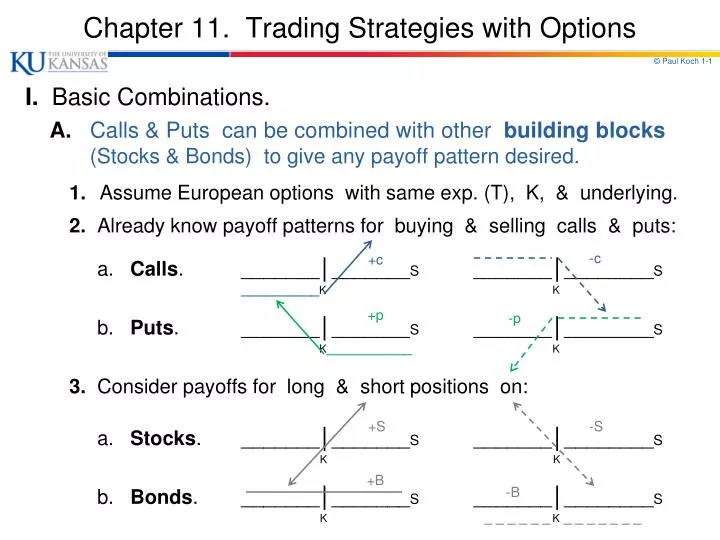
Chapter 11. Trading Strategies with Options. I. Basic Combinations. A . Calls & Puts can be combined with other building blocks ( Stocks & Bonds) to give any payoff pattern desired. 1. Assume European options with same exp. (T), K, & underlying.

E N D
Chapter 11. Trading Strategies with Options I. Basic Combinations. A.Calls & Puts can be combined with other building blocks (Stocks & Bonds) to give any payoff pattern desired. 1.Assume European options with same exp. (T), K, & underlying. 2. Already know payoff patterns for buying & selling calls & puts: a. Calls. _______│_______S _______│________S __________KK b. Puts. _______│_______S _______│________S K___________K 3. Consider payoffs for long & short positions on: a. Stocks. _______│_______S _______│________S KK b. Bonds. _______│_______S _______│________S K _ _ _ _ _ _K _ _ _ _ _ _ _ -c +c +p -p +S -S +B -B
I.B. Protective Put (S+P) B. Buy Stock (+S) and Buy Put (+P) Value +S +P S+P S
I.C. Principal - Protected Note* (B+C) C. Buy Bond (+B) and Buy Call (+C) * If you buy a zero-coupon, deep discount bond, the initial outlay (B) is small (esp. if r is high); If volatility of S is low, call (C) is cheap; Then the initial cost (B+C) may be set ≈ K (PPN). Then your principal is protected (worst outcome; S low, call OTM, get to keep Bond payoff (K). Value +B +C B+C S
I.D. Put-Call Parity (S+P = B+C) D. B & C give same payoff pattern (S+P = B+C) Value +S +P S+P +B +C B+C S
I.E. Writing a Covered Call (+S - C) E. Buy Stock (+S) and Sell Call (-C) +S Value -C S-C S+P = B+C ↓ S-C = B-P S
I.F. Buying a Straddle (+C+P) F. Buy Call (+C) and Buy Put (+P) Value +C +P C+P S
I.G. Selling a Straddle (-C-P) G. Sell a Call (-C) and Sell a Put (-P) Value -C -P -C-P S
I.H. Buying a Strangle (+C+P) – with Different K’s H. Buy Call with K2; Buy Put with K1 (K1 < K2) Value +C2 +P1 C2+P1 S K2 K1
II. How to Plot Payoff Pattern for Any Combination Problem: Given any Combination of shares, bonds, & options, graph the Payoff Pattern for the Intrinsic Value; show slopes of line segments; & show break-even points. Three Steps: 1. Compute the initial cost / revenue of the Combination, and get values of S where all options are worth zero (ATM or OTM). For these values of S, Combination is worth the initial cost / revenue. 2. Get values of S where one option is ITM. For these values of S, Combination Value = initial cost / revenue + intrinsic value of this option. 3. Get values of S where next option is ITM. For these values of S, Combination Value = old value + intrinsic value of this option. Continue until you examine all values of S, for all options in combination.
II. How to Plot Payoff Pattern for Any Combination Example 1: Strip; Buy 1 Call & 2 Puts with same K = $50; C = $5; P = $6. 1. Initial Cost = (-1) x ($5) + (-2) x ($6) = -$17. At S = K = $50, both options ATM, Combination Value = -$17. 2. If S > $50, Call ITM, Combination Value = -$17 + 1(S - K). (coeff. of S = +1) 3. If S < $50, Puts ITM, Combination Value = -$17 + 2(K - S). (coeff. of S = -2) K = $50 ____________________________________________________________ S $41.50 │ $67 │ │ │ slope = -2 │ slope = +1 │ │ │ │ -17│ │
II. How to Plot Payoff Pattern for Any Combination Example 2:Buy 1 Call with K1 = $40 (C1 = $8); Sell 2 Calls with K2 = $45 (C2 = $5). 1. Initial Cost = (-1) x ($8) + (+2) x ($5) = +$2. If S < K1 = $40, both options OTM, Combination Value = +$2. (coeff of S = 0) 2. If 40 < S < $45, C1 is ITM, Value = +$2 + 1(S - K1). (coeff = +1) 3. If S > $45, C1 & C2 are ITM, Value = +$2 + 1(S - K1) - 2(S - K2). (coeff = -1) K = $40 K = $45 │ 7│ │ │ slope = +1 │ │ slope = -1 2│ slope = 0│ _____________________________________________________ S │ $45$52 │
II.A. Bull Spread with Calls (C1 - C2) A.Buy Call with K1 (pay C1); Sell Call with K2 (receive C2) (K1< K2); Thus (C1 > C2); So (-C1 +C2) < 0; initial outflow (left) Value +C2 S K2 K1 (-C1+C2) -C1
II.B. Bull Spread with Puts (P1 - P2) B.Buy Put with K1 (pay P1); Sell Put with K2 (receive P2) (K1 < K2); Thus (P1 < P2); So (-P1 +P2) > 0; initial inflow (right) Value (-P1+P2 ) +P2 S K1 -P1 K2
II.C. Bear Spread with Calls (C2 - C1) C. Sell Call with K1 (receive C1); Buy Call with K2 (pay C2) (K1 < K2); Thus (C1 > C2); So (+C1 -C2) > 0; initial inflow (left) Value (+C1 -C2) C1 S C2 K1 K2
II.D. Bear Spread with Puts (P2 - P1) D. Sell Put with K1 (receive P1); Buy Put with K2 (pay P2) (K1 < K2); Thus (P1 < P2); So (+P1 -P2) < 0; initial outflow (right) Value P1 S K1 K2 (+P1 -P2) P2
II.E. Butterfly Spread with Calls (C1 - 2C2 + C3) E.Buy 1 Call with K1; Sell 2 Calls with K2; Buy 1 Call with K3 (K1 < K2 < K3); Thus, (C1> C2 > C3); initial outflow (left).
II.F. Butterfly Spread with Puts (P1 - 2P2 + P3) F.Buy 1 Put with K1; Sell 2 Puts with K2; Buy 1 Put with K3 (K1 < K2 < K3); Thus, (P1 < P2 < P3); initial outflow (right).
III.A. Graphing Total, Intrinsic, and Extrinsic Value 0 < dc/dS < 1 Total Value If σ↑ dc/dS = 1 S K dc/dS = 0 Intrinsic Value S K Extrinsic Value S K
III.B. Buy Calendar Spread using Calls (+C2 - C1) B. Buy Call with maturity, T2 ; Sell Call with maturity, T1 ; (T2 > T1); Thus, (C2 > C1); initial outflow.
III.C. Buy Calendar Spread using Puts (+P2 - P1) C.Buy Put with maturity, T2 ; Sell Put with maturity, T1 ; (T2 > T1); Thus, (P2 > P1); initial outflow.
IV. Interest Rate Option Combinations (Hull Chap 21) A. Using Options on Eurodollar Futures. 1. ED Futures Contract Characteristics : (Review) a. Underlying Asset - ED deposit with 3-month maturity. b. ED rates are quoted on an interest-bearing basis, assuming a 360-day year. c. Each ED futures contract represents $1MM of face value ED deposits maturing 3 months after contract expiration. d. 40 different contracts trade at any point in time; contracts mature in Mar, Je, Sept, and Dec, 10 years out. e. Settlement is in cash; price is established by a survey of current ED rates. f. ED futures trade according to an index; Q = 100 - R = 100 - (futures rate); e.g., If futures rate = 8.50%, Q = 91.50, and interest outlay promised would be (.0850) x ($1,000,000) x (90 / 360) = $21,250. g. Each basis point in the futures rate means a $25 change in value of contract: [ (.0001) x ($1,000,000) x (90 / 360) ] = $25 ] h. The ED futures is truly a futures on an interest rate. (The T.Bill futures is a futures on a 90-day T.Bill.)
IV.A. Using Options on ED Futures 2. Example: Long Hedge with ED futures for a Bank. (more Review) Jan. 6: Bank expects $1 MM payment on May 11 (4 months). Anticipates investing funds in 3-month ED deposits. Cash Market risk exposure: Bank would like to invest @ today’s ED rate, but won’t have funds for 4 mo. If ED rate , bank will realize opportunity loss (will have to invest the $1 MM at lower ED rates). Long Hedge: Buy ED futures today (promise to deposit later @ R). Then if cash rates , futures rates (R) will & futures prices (Q) will . so long futures position will to offset opportunity losses in cash mkt. The best ED futures to buy is June contract; expires soonest after May 11. Jan. 6 May 11 June 14 |__________________________________________|_____________| $1 MM receivable due May 11. Cash: Plan to invest $1MM on May 11 Invest the $1 MM in ED deposits. Futures: Buy 1 ED futures. Sell futures contract.
IV.A. Using Options on ED Futures 3. Data for example – (more Review) Jan. 6: Cash market ED rate (LIBOR) = RS = 3.38% (S1 = 96.62) June ED futures rate (LIBOR) = RF = 3.85% (F1 = 96.15) ; Basis = (S1 - F1) = .47% May 11: Cash market ED rate = 3.03% (S2 = 96.97) June ED futures rate = 3.60% (F2 = 96.40) ; Basis = (S2 - F2) = .57%_______________________________________________________________________________ Date Cash Market Futures Market Basis 1 / 6 bank plans to invest $1MM bank buys 1 Je ED futures at cash rate = S0 = 3.38% at futures rate = R0 = 3.85%.47% 5 / 11 bank invests $1MM in 3-mo ED bank sells 1 June ED futures at cash rate = S1 = 3.03% at futures rate = R1 = 3.60%.57% Net opport. loss = 3.38 - 3.03 = .35%futures gain = 3.85 - 3.60 = .25% change Effect (35) x ($25) = $875 (25) x ($25) = $625 .10% . Cumulative Investment Income: Interest @ 3.03% = $1,000,000 (.0303) (90/360) = $7,575 Profit from futures trades: = $625 Total: $8,200 Effective Return = [ $8,200 / $1,000,000 ] x (360 / 90) = 3.28% (10 bp worse than spot market = change in basis). This is basis risk.
IV.A. Using Options on ED Futures 4. Using Options on ED futures to build Floors, Caps, & Collars. a. ED futures contract: Buy ; Promise to buy ED ( lend @ forward ED rate); Sell ; Promise to sell ED (borrow @ forward ED rate). [ Lock in R. ] b. Call option on ED futures: Rightto buy ED futures (lend @ forward ED rate). c. Put option on ED futures: Right to sell ED futures (borrow @ fwd ED rate). d. Lender? Want to buy ED in future. To hedge risk of loss with falling rates: i. Buy ED futures. If rates , lock in (min.) lending rate. But if rates , opportunity loss (could have loaned at higher rates). ii. Buy Call option on ED futures. If rates , lock in min. lending rate. NOW if rates , lend at higher rates! Call is OTM - interest rate Floor. e. Borrower?Want to sell ED in future. To hedge risk of loss with rising rates: i. Sell ED futures. If rates , lock in (max.) borrowing rate. But if rates , opportunity loss (could have borrowed at lower rates). ii. Buy Put option on ED futures. If rates , lock in max. borrowing rate. NOW if rates , borrow at lower rates! Put is OTM - interest rate Cap. f. Combining Call & Put on ED futures gives Collar.
IV.A. Using Options on ED Futures 5. Example: Building Interest Rate Collar for a bank. Cap: Buy a Put.Floor: Sell a Call . Both: Collar . Strike Option Strike Option Range of Net Price Premium Price Premium Borrowing Cost Premium . 96.00 .13 96.75 .02 3¼% - 4% .11 = $275 96.50 .40 96.75 .02 3¼% - 3½% .38 = $950 96.25 .23 96.50 .05 3½% - 3¾% .18 = $450 . Cap at 4%; Floor at 3¼ %; Collar: Net Cost = 11 basis points. | | | 96.00 96.75 |> Futures Price (Q) | | | Loss a. CAP borrowing rates @ 4% by buying a Put with K = 96.00 (= 100 - 4). Must pay 13 bp for this Put (13 x $25 = $325). i. If ED rates above 4%, Q below 96.00, & Put is ITM – Cap at 4%. ii.If ED rates below4%, Q above96.00, & Put is OTM– Borrow at < 4%. b. If you don’t think ED rates will below, say, 3.25%, can recover some of cost by selling a Callwith K = 96.75 (= 100 - 3.25). Receive 2 bp ($50). i. If ED rates below 3.25%, Q above 96.75%, & Call is ITM – Floor at 3.25%. Sell call 0.02 0.11 0.13 Buy put