Download
1 / 15
150 likes | 210 Views
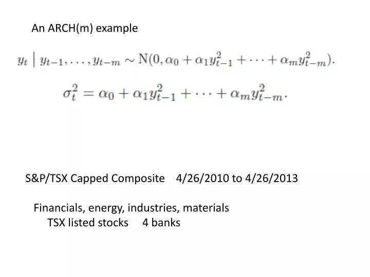
An ARCH(m) example. S&P/TSX Capped Composite 4/26/2010 to 4/26/2013 Financials, energy, industries, materials TSX listed stocks 4 banks. r ate log (ratio) volatility smo (y) lowess (y) lowess (|y – smo (y)|

E N D
An ARCH(m) example S&P/TSX Capped Composite 4/26/2010 to 4/26/2013 Financials, energy, industries, materials TSX listed stocks 4 banks
rate log (ratio) volatility smo(y) lowess(y) lowess(|y – smo(y)| library(tseries)junk0<-scan("SPTXT.txt")p<-rev(junk0)y<-diff(log(p))ny<-length(y)par(mfrow=c(2,1))xaxis<-1:nyy<-ts(y,start=1,end=ny)plot(y,main="SPTXT 2010 to 2013",xlab="trading day",ylab="return")lunk<-lowess(xaxis,abs(y-mean(y)),f=.001)yabs<-ts(lunk$y,start=1,end=ny)plot(yabs,main="Smoothed abs(deviation)",xlab="trading day",ylab="")
acf, pacf ARCH? par(mfrow=c(2,1))acf(y,main="ACF SPTXT returns",xlab="lag (days)")yy<-y-mean(y);yy<-yy^2pacf(yy,main="PACF SPTXT returns^2",xlab="lag (days)")
Fitted conditional variance useful in forecasting plugin estimate of library(tseries)P<-5PP<-P+1junk1<-garch(y,order=c(0,P),grad="analytic")summary(junk1)par(mfrow=c(2,1))yvol<-ts(junk1$fit[,1],start=1,end=ny)plot(yvol,type="l",ylim=c(0,max(abs(y))),main=paste("Estimated volatility - ARCH",P),xlab="trading day",ylab="volatility") Standardized residuals yres<-ts(junk1$res,start=1,end=ny)
one step ahead cdl se standardized
Standardized residuals yres<-ts(junk1$res,start=1,end=ny)plot(yres,main="Residuals of ARCH(5)",type="l",xlab="trading day",ylab="return")
plot(junk1$coef[2:PP],type="l",las=1,main="Coefficients",ylim=c(0,max(junk1$coef[2:PP])),ylab="coef")plot(junk1$coef[2:PP],type="l",las=1,main="Coefficients",ylim=c(0,max(junk1$coef[2:PP])),ylab="coef") ave<-mean(junk1$coef[2:PP]) abline(h=ave) junk1$asy<-sqrt(diag(junk1$vcov)) lines(ave+junk1$asy,lty=3) lines(ave-junk1$asy,lty=3)