Download

1 / 36
360 likes | 441 Views
Numerical ‘black hole’ simulations. Luis Lehner LSU [NSF-NASA-Sloan-Research Corporation]. Overview. Status of ‘basic’ efforts What we know & would like to know at continuum level From continuum to discrete Head-ways/messages to other disciplines

E N D
Numerical ‘black hole’ simulations Luis Lehner LSU [NSF-NASA-Sloan-Research Corporation]
Overview • Status of ‘basic’ efforts • What we know & would like to know at continuum level • From continuum to discrete • Head-ways/messages to other disciplines • Status through 3 examples (3,2,1 + time dimensions). From ‘qualitative’ to precision physics…. • Astrophysical black hole simulations • Higher dimensional black holes and related systems • Final comments
Where are we now‘The good, the bad and the ugly’ • Initial value problem: Advanced on development, analysis and use of formulations of Einstein equations. • Previously used equations were weakly hyperbolic generically ill-posed! • Can be ‘fixed’ by adding constraints (and coord conditions) in a suitable manner • Yet, lots of possibilities, ‘infinitely’ many different formulations. • Poor’s man way: parameter search, dynamical adjusting them, and/or ‘clean-up’ constraints. Tiglio,LL,Neilsen
Initial value boundary problem: Well posedness established [Friedrich-Nagy]. • Allows for specifying the ‘right’ boundary –physical– data. Just one formulation where this is known at the non-linear level • A couple of others at linear level, well posed but unable to specify desired boundary condition • Poor’s man way of dealing with this: Push boundaries far out. • A more refined way, understand well posedness of underlying problem with suitable boundary conditions. For radiative ones, in a standard formulation elliptic gauge equation to rule out weak (polynomial) instability [Sarbach-Reula in a model problem]. • For global problem. Reach future null infinity by matching formulations or conformal eqns.
Moving to numerical arena • Guiding principle: reproduce analytical steps at ‘all’ cost. • System: • What’s involved here? • Why did we get this? • Numerically? Obtain a (semi-) discrete energy estimate • Operator? • Boundaries? • Dissipation? • Integration in time. RK3-RK4 preserves the discrete energy stability! Gustaffson-Kreiss-Oliger; Strand; Olsson; Tadmor Calabrese-L.L.-Neilsen-Pullin-Reula-Sarbach-Tiglio
Example 1 • Binary black hole simulations. • Leading edge, a few efforts leading to ‘orbits’. • Rationale, use what is available the ‘best’ possible way and push ahead the problem at hand. • F. Pretorius effort: • Einstein eqns in harmonic coordinates. • Adaptive mesh refinement to achieve high resolution near black holes • Addition of constraint terms to ‘damp’ spurious growth. [H. Friedrich, Sarbach-Tom]
Generalized harmonic coordinates introduce a set of arbitrary source functionsH u into the usual definition of harmonic coordinates • With H u regarded as independent functions, the principle part of the equation for each metric element reduces to a simple wave equation • Constraints: • Behavior? • To help with constraint’s growth, modify eqns by adding constraints [Gundach et al, following Brodbeck-Huebner-Reula-Frittelli]
Effect of damping terms • Axisymmetric simulation of a Schwarzschild black hole, Painleve-Gullstrand coords. • Left and right simulations use identical parameters except for the use of constraint damping • Not ‘robust’ for al problems
status, prospects…. • ‘Realistic’ initial data still unknown, presently trying to understand generic features of binary black hole mergers • Initial data defined by boosted over-critical scalar field configurations. • choice for initial geometry and scalar field profile: • spatial metric and its first time derivative is conformally flat • maximal (gives initial value of lapse and time derivative of conformal factor) and harmonic (gives initial time derivatives of lapse and shift) • Hamiltonian and Momentum constraints solved for initial values of the conformal factor and shift, respectively • advantages of this approach • “simple” in that initial time slice is singularity free • all non-trivial initial geometry is driven by the scalar field—when the scalar field amplitude is zero he recovers Minkowski spacetime • disadvantages • ad-hoc in choice of parameters to produce a desired binary system • uncontrollable amount of “junk” initial radiation (scalar and gravitational) in the spacetime; though all present initial data schemes suffer from this to some degree. • Numerical ingredients • Adaptive mesh refinement technique employed • ‘Compactification’ of spatial coordinates + artificial dissipation to wipe out everything that leaves sufficiently far.
‘dynamics’ • Initially: • equal mass components • eccentricity e ~ 0 - 0.2 • coordinate separation of black holes ~ 13M • proper distance between horizons ~ 16M • velocity of each black hole ~0.16 • spin angular momentum = 0 • ADM Mass ~ 2.4M • Final black hole: • Mf~ 1.9M • Kerr parameter a ~ 0.70 • ‘error’ ~ 5%
Scalar field f.r, uncompactified coordinates Scalar field f.r, compactified (code) coordinates
Simulation (center of mass) coordinates Reduced mass frame; heavier lines are position of BH 1 relative to BH 2 (green star); thinner black lines are reference ellipses
Real component of the Newman-Penrose scalar Y4times r,x=0 slice of the solution Real component of the Newman-Penrose scalar Y4times r,z=0 slice of the solution
Summary of computation – medium resolution simulation • base grid resolution 333 • 9 levels of 2:1 mesh refinement (effective finest grid resolution of 81923) … switched to 8 levels maximum at around 150M • ~ 50,000 time steps on finest level • ~550 hours on 48 nodes of UBC’s vnp4 Xeon cluster (26,000 CPU hours total) • maximum total memory usage ~ 10GB, disk usage ~ 100GB (and this is very infrequent output!)
Pushing ahead… Zoom-whirl ? finite number of ‘humps’
Notes…. • ‘First-sight’ prognosis… bbh orbits underway. Some qualitative, semi-quantitative answers coming and in the way. • Estimates of expected growth can play a major role: • to discern among different formulations • to exploit this knowledge at the numerical level • How must one deal with ‘non-constant’ characteristic structure? • e.g. u,t=f(x,y) u,x with f(x=0,y) = sin(y) • Existing/gained knowledge spilling out to close fields • Eg. MHD eqns often used are weakly hyperbolic, upon re-expression yield vastly improved simulations without ‘special tricks’ [Hirschman-Neilsen-Reula-LL] • Every simulation still require large resources – too long times– . Further developments in numerics/computational techniques to come.
Black strings and bubbles • Black strings: higher dimensional black holes. In 5D black holes with ‘maximum’ symmetries are : S3 hyperspherical black hole or S2xR cylindrical black hole or black string. • Bubbles. Topogically ‘weird’ spacetimes. • An initially large sphere can’t be shrank to zero size • Minkowski spacetime shown to be able to ‘quantum tunnel’ to a bubble spacetime (Witten bubble) • Studying both systems require numerical simulations of Einstein equations in higher dimensions (5D) but symmetries allow for treating the black string in 2+1 and bubble in 1+1 dimensions.
Black strings 1.- Contain singularities 2.- Ruled by null-rays 3.- Non-unique even in spherical symm Stability? - Black string perturbations admit exponential growth for L > Lc (Gregory-Laflamme) - Entropy SBS<SBH(for a given M) Conjecture: Black strings will bifurcate
Conjecture used in many scenarios • Density of states from Ads/CFT correspondence • Discussions of BH on brane worlds. BH in matrix theory, etc • Recent developments • Horowitz-Maeda, can’t bifurcate in finite time. Conjecture: will ‘settle’ to a non-uniform stationary soln (ie. No bifurcation in infinite affine time) • Gubser: transition to soln of first-order type in 5-6D (1st, ~2nd order pert) • Wiseman: stationary solns which are not the Horowitz-Maeda ones. • Kol: Transition from black string to BH through a conical singularity • Sorkin-Kol: for high enough dimensions transition is of 2nd order. • Qns: • What is the final solution of a perturbed black string? • Can it bifurcate in ‘infinite time’? • Are Wiseman’s solns, physically relevant?
Some details • Spherical symmetry 2+1 problem. BUT a priori quite a zoo of possibilities! • Line element: • Initial data • Solve constraints with a seed perturbation in gqq • Boundary? • Might need to ‘evolve’ for very long!. ‘Compactify’ r direction (dissipation needed)
Monitoring the evolution • Apparent horizon & Null surfaces • Kretschmann invariant I=Rabcd Rabcd • For BS, at ev. horizon: IA = 12/R4 ; • For hyperspherical BH at ev horizon: IA = 72/R4 • Monitor I R4/12 {1,6} for {BS, hyper.BH} • Excision at: • RAH – buffer • min(RAH) – buffer • Radial resolution near app horizon ~ M/(200 x n) {n=1..8} Checked evolution independence on choice made [Choptuik,LL,Olabarrieta,Pretorius,Petryk,Villegas]
Curvature ‘Event’ horizon
Affine time, l=es growing exponentially (~1022) • “bifurcation” in infinite affine time certainly possible • ‘cascade’ of unstable strings also possible [Garfinkle-LL-Pretorius]
Problem: Kaluza-Klein ‘bubbles’ • Positive mass thm (Witten) requires existence of certain (asymptotically constant) spinors. In 5d Kaluza-Klein theory (asymptotically R3xS1) these spinors are not guaranteed. • Are there negative mass configurations? • Is cosmic censorship valid? • Answer to 1. Yes, negative mass configurations found • Witten bubble (82): associated with instability of KK vacuum. More than 1 state with zero total energy. • Brill-Pfister (89): explicit solutions to 5D vacuum constraints with negative mass. • Brill-Horowitz (91): generalization to include ‘gauge’ fields. • Qn: What’s the space-time like? • Corley-Jacobson (94). Analyze area of the bubble, conclusion: It starts out expanding [collapsing], if this trend continues, unlikely to form a singularity. • Conjecture: It will keep expanding [collapsing] out (otherwise go through another moment of time symmetry). • But….. This only from estimates at the initial hypersurface… what does really happen?… Need to solve the eqns… • Numerical effort (2000). Conclusion: negative mass bubbles expand but not forever…. At some point a naked singularity appears!!! (or does it?)
Revisiting the problem • Consider: • With U(r) 0 (for r=r+ ) a smooth function (U1 asymptotically) • Bubble is at r+. • Electrovac case, consider • Time symmetry (mom const =0); Hamiltonian constraint • With m,b constants. In particular MADM=m/4…but this can be negative • Initial acceleration of the bubble’s area [extending Corley-Jacobson] • n=2. If m<0, bubble expands; m>0 both cases possible • n>2. For k large, arbitrary negative acceleration with negative mass…sounds promising! Sarbach, LL PRD 03; 05.
Numerical evolution • Variables functions of (t,r) only (1D evolution) • Understood constraint growth and suitable boundary conditions [a-la Calabrese,LL,Tiglio 02] • At bubble, regularity conditions used. • Proved well posedness at continuum level, translated to the numerical arena thanks to SBP in a first order formulation. • Improved resolution at bubble with a non-uniform radial coordinate. k=0 Case studied numerically previously, no naked singularity found, m<0 expands even faster than m>0
More than we asked for… • What happens with a non-zero gauge field? • Choose n=2, and stick to cases where bubble starts out collapsing (positive mass) Depending on field strength, the bubble either collapses (k<k*) to a black string or bounces back to expand (k>k*). Changes behavior almost always without going through another moment of time symmetry Last… it appears to approach a stationary solution… does it exist?
Curvature invariant, sub/supra critical behavior Observation… there must be a static solution at the threshold
Put static anzats, solve resulting constraint and… • With V=(1-r-/r); U=(1-r+/r). And the parameters are obtained from • P=4pr+(1-r-/r+)(3/2) and M=r+/4. • New solution?… nah… obtained by ‘just’ analytically continuing that of a charged black string….[found in Horowitz-Maeda 03] • Analyzed spectrum of operator and confirmed a • single growing mode f ~ ekt • Pulsation operator, upper/lower bounds within a • suitable Hilbert space, Sturm-Liouville type problem • Upon : tiz, zit f ~ eikz, k ~ 1/Lc • Used to show a family of charged black strings becomes more unstable as charged is added (opposite to what was conjectured)
What happened with the negative mass data that started contracting with arbitrary negative acceleration? • Bubble shrinks to arbitrarily small sizes, but ‘bounces’ back… cosmic censorship stood its ground
Final words • Numerical relativity can indeed provide ‘experimental’ set-up and pose new questions • Critical phenomena • Cosmology • Bubble/black string problem • Robust ‘generic’ implementations of Einstein equations will benefit (a lot!) from extra input ‘analytically’ obtained • Estimates including lower order terms (problem dependent, but technique?) • Estimates including constraint growth (or how to control them) • Constraint preserving boundary conditions or how to go around them • Radiative boundary conditions (no theory so far), how to proceed with non-constant characteristics? • Translation of the above to numerics, implementation, resolution, etc + all the ‘extra-can-of-worms’ that come with this. • In the mean time, we’ll do the best we can!