Download

1 / 104
1.05k likes | 1.28k Views
Using Basic Formulas and Functions. Lesson 8. Objectives. Software Orientation: Formulas Tab. In this Lesson, you’ll use command groups on the Formulas tab, as shown in the figure. These commands are your tools for building formulas and using functions in Excel.

E N D
Using Basic Formulas and Functions Lesson 8
Software Orientation: Formulas Tab • In this Lesson, you’ll use command groups on the Formulas tab, as shown in the figure. These commands are your tools for building formulas and using functions in Excel. • Use this illustration as a reference throughout this lesson as you become familiar with the command groups on the Formulas tab and use them to create formulas.
Building Basic Formulas • The real strength of Excel is its ability to perform common and complex calculations. • A formula is an equation that performs calculations, such as addition, subtraction, multiplication, and division, on values in a worksheet. • When you enter a formula in a cell, the formula is stored internally and the results are displayed in the cell. • Formulas give results and solutions that help you assess and analyze data.
Creating a Formula that Performs Addition • A formula consists of two elements: operands and mathematical operators. • Operands identify the values to be used in the calculation. An operand can be a constant value, a cell reference, a range of cells, or another formula. A constant is a number or text value that is entered directly into a formula. • Mathematical operators specify the calculations to be performed. To allow Excel to distinguish formulas from data, all formulas begin with an equal sign (=). • In the next exercise, you will learn how to create basic formulas that perform mathematical computations and apply the formulas using various methods.
Creating a Formula that Performs Addition • When you build a formula, it appears in the formula bar and in the cell itself. • When you complete the formula and press Enter, the value displays in the cell and the formula displays in the formula bar. • You can edit a formula in the cell or in the formula bar the same way you can edit any data entry.
Step-by-Step: Create a Formula for Addition • Before you begin these steps, LAUNCH Microsoft Excel and OPEN a blank workbook. • Select A1 and key =25+15. Press Tab. Excel calculates the value in A1, and displays the sum of 40 in the cell. • In B1, key +18+35. Press Tab. The sum of the two numbers, 53, appears in the cell. NOTE: Formulas should be keyed without spaces, but if you key spaces, Excel eliminates them when you press Enter.
Step-by-Step: Create a Formula for Addition • Select B1 to display the formula for that cell in the formula bar. As illustrated in the figure below, although you entered + to begin the formula, when you pressed Enter, Excel replaced the + with = as the beginning mathematical operator. This is the Excel formula auto correct feature.
Step-by-Step: Create a Formula for Addition • Select A3. Click the formula bar and key =94+89+35. Press Enter. The sum of the three numbers, 218, appears in the cell. • Select A3 and click the formula bar. Select 89 and key 98. Press Enter. Notice that your sum changes to 227. • LEAVE the workbook open to use in the next exercise.
Creating a Formula that Performs Subtraction • The same methods you used to create a formula to perform addition can be used to create a formula to perform subtraction. • When you create a subtraction formula, enter = followed by the positive number and then enter a minus sign to indicate subtraction. When you create a subtraction formula, the minus sign must precede the number to be subtracted. • In the next exercise, you practice creating a formula that performs subtraction.
Creating a Formula that Performs Subtraction • When you enter a formula to subtract 125 from 189, you could enter =189−125 or = −125+189. Either formula yields a positive 64. If the positive number is entered first, it is not necessary to enter a plus sign. • If you find that you’ve made a mistake in your formula (such as returning the negative number mentioned earlier), you can select the cell with the erroneous function, press F2 to take you to the formula bar, and edit your function. Once you’ve made your corrections, press Enter to revise.
Step-by-Step: Create a Formula for Subtraction • USE the workbook from the previous exercise. • Select A5. Key =456−98. Press Enter. The value in A5, 358, appears in the cell. • Select A6 and key =545−13−8. Press Enter. The value in A6 should be 524. • In A8, create a formula to subtract 125 from 189. The value in A8 should be 64. • LEAVE the workbook open to use in the next exercise.
Creating a Formula that Performs Multiplication • The formula to multiply 33 by 6 is =33*6. • If a formula contains two or more operators, operations are not necessarily performed in the order in which you read the formula. • The order is determined by the rules of mathematics, but you can override standard operator priorities by using parentheses. • Operations contained in parentheses are completed before those outside parentheses. • In the next exercise, you learn to create formulas that perform multiplication.
Step-by-Step: Create a Formula for Multiplication • USE the workbook from the previous exercise. • Select D1. Key =125*4 and press Enter. The value that appears in D1 is 500. • Select D3 and key =2*7.50*2. Press Enter. The value in D3 is 30. • Select D5 and key =5*3. Press Enter. The value in D5 is 15. • Select D7 and key =5+2*8. The value in D7 is 21. • Select D9 and key =(5+2)*8. The value in D9 is 56. • LEAVE the workbook open to use in the next exercise.
Creating a Formula that Performs Division • The forward slash is the mathematical operator for division. • When a calculation includes multiple values, you must use parentheses to indicate the part of the calculation that should be performed first.
Creating a Formula that Performs Division • Excel does not necessarily perform the operations in the same order that you enter or read them in a formula, which is left to right. Excel uses the rules of mathematics to determine which operations to perform first when a formula contains multiple operators. This is also known as the order of evaluation in Excel. The order is: • negative number (−) • percent (%) • exponentiation (ˆ) • multiplication (*) and division (/) • addition (+) and subtraction (−)
Creating a Formula that Performs Division • For example, consider the following equation: 5 + 6 * 15 / 3 −1 = 34 • Following mathematical operator priorities, the first operation would be 6 multiplied by 15 and that result would be divided by 3. Then 5 would be added and finally, 1 would be subtracted. The figureillustrates the formula entered into Excel.
Creating a Formula that Performs Division • When you use parentheses in a formula, you indicate which calculation to perform first, which overrides the standard operator priorities. Therefore, the result of the following equation would be significantly different from the previous one. The figure illustrates the Excel formula. • Here is the mathematical formula: (5 + 6) * 15 / (3 −1) = 82.5
Step-by-Step: Create a Formula for Division • USE the workbook from the previous exercise. • Select D7 and create the formula =795/45. Press Enter. Excel returns a value of 17.66667 in D7. • Select D7. Excel applied the number format to this cell when it returned the value in step 1. Click the Accounting Number Format ($) button, on the Home tab in the Numbers group, to apply accounting format to cell D7. The number is rounded to $17.67 because two decimal places is the default setting for the accounting format.
Step-by-Step: Create a Formula for Division • Select D9 and create the formula =65−29*8+97/5. Press Enter. The value in D9 is −147.6. • Select D9. Click in the formula bar and place parentheses around 65–29. Press Enter. The value in D9 is 307.4. • CLOSE but do not save the workbook. • LEAVE Excel open to use in the next exercise.
Using Cell References in Formulas • A cell reference in a formula identifies a cell or a range of cells on a worksheet and tells Excel where to look for the values you want it to calculate in the formula. • Using cell references (cell names; A1, B1, and so on) enables you to re-use the formulas you write, by updating the data in the formulas, rather than rewriting the formulas themselves. • With references, you can use values contained in different parts of a worksheet in one formula or use the value from one cell in several formulas. You can also refer to cells on another worksheet in the same workbook, as well as to other workbooks. • Excel recognizes two types of cell references—relative and absolute.
Using Relative Cell References in a Formula • A cell reference identifies a cell’s location in the worksheet, based on its row number and column letter. • When you include a relative cell reference in a formula and copy that formula, Excel changes the reference to match the column or row to which the formula is copied. A relative cell reference is, therefore, one whose references change “relative” to the location where it is copied or moved. • You use relative cell references when you want the reference to automatically adjust when you copy or fill the formula across rows or down columns in ranges of cells. By default, new formulas use relative references. • In the next exercise, you practice creating and using relative cell references in formulas.
Using Relative Cell References in a Formula • You are about to learn two methods for creating formulas using relative references: • By keying in an equal sign to mark the entry as a formula and then keying the formula directly into the cell; and • By keying an equal sign and then clicking a cell or cell range included in the formula (rather than keying cell references). • The second method is usually quicker and eliminates the possibility of typing an incorrect cell or range reference. • When you complete the formula and press Enter, the value displays in the cell and the formula displays in the formula bar.
Step-by-Step: Use Relative Cell References • LAUNCH Microsoft Excel if it is not already open. • OPEN the Personal Budget data file for this lesson. • Select B7 and key =sum(B4: (colon). As shown in the figure, cell B4 is outlined in blue, and the reference to B4 in the formula is also blue. The ScreenTip below the formula identifies B4 as the first number in the formula. The reference to B4 is based on its relative position to B7, the cell that contains the formula.
Step-by-Step: Use Relative Cell References • Key B6 and press Enter. The total of the cells, 3,760, appears in B7. • Select B15. Key =sum( and click B10. As shown in the figure, B10 appears in the formula bar and a flashing marquee appears around B10. Excel now knows that you are selecting thiscell to be used in the formula.
Step-by-Step: Use Relative Cell References • Click and drag the flashing marquee to B14. As shown in the figure, the formula bar reveals that values within the B10:B14 range will be summed (added). Note, this step allows you to input a range ofcells in the formula by highlighting instead of typing the formula in the cell.
Step-by-Step: Use Relative Cell References • Press Enter to accept the formula. Select B15. As illustrated in the figure, the value is displayed in B15 and when you click on the cell the formula is displayed in the formula bar. Take note that each cell reference is the cell’s unique name. No matter what numeric value is assigned in the cell, the cell reference (B1, C10,etc.) never changes.
Step-by-Step: Use Relative Cell References • The goal of this step is to create a simple formula. Select D4 and key =. Click B4 and key −. Click C4 and press Enter. By default, when a subtraction formula yields no difference (a zero answer), Excel enters a hyphen. • Select D4 again. Click and drag the fill handle to D7 to select this range of cells. You are now copying the formula from the previous step into a new range of cells. • Use the fill handle to copy the formula in B7 to C7. Notice that the amount in D7 changes when the formula is copied. When you copied the formula to C7, the position of the cell containing the formula changed, so the reference in the formula changed to C7 instead of B7.
Step-by-Step: Use Relative Cell References • Select D7 and click Copy. Select D10:D15 and click Paste. Your formula is copied to the range of cells and Excel has automatically adjusted the cell references accordingly. Note that D7 is still highlighted by the flashing marquee. • Select D17:D21 and click Paste. Your formula from D7 is now copied to the second range of cells and the references are adjusted. Note that the flashing marquee is still surrounding D7. You have the ability to copy one formula into multiple locations without having to recopy it. • Create a Lesson 8 folder and SAVE your worksheet as Budget. • LEAVE the workbook open to use in the next exercise.
Using Absolute Cell References in a Formula • Sometimes you do not want a cell reference to change when you move or copy it. For example, when you review your personal budget, you might want to know what percentage of your income is budgeted for each category of expenses. • Each formula you create to calculate those percentages will refer to the cell that contains the total income amount. • The reference to the total income cell is an absolute cell reference—a reference that does not change when the formula is copied or moved.
Using Absolute Cell References in a Formula • Absolute cell references include two dollar signs in the formula. • The absolute cell reference $B$7 in this exercise, for example, will always refer to cell B7 because dollar signs precede both the column (B) and row (7). • When you copy or fill the formula across rows or down columns, the absolute reference will not adjust to the destination cells. • By default, new formulas use relative references, and you must edit them if you want them to be absolute references.
Using Absolute Cell References in a Formula • You can also create a mixed reference in which either a column, or a row, is absolute or the other is relative. For example, if the cell reference in a formula were $B7 or B$7, you would have a mixed reference in which one component is absolute and one is relative. • The column is absolute and would remain unchanged in the formula, and the row is relative if the reference is $B7, changing as the mixed reference is copied to $B7, $B8, and so on.
Using Absolute Cell References in a Formula • If you copy or fill a formula across rows or down columns, the relative reference automatically adjusts, and the absolute reference does not adjust. For example, if you copied or filled a formula containing the mixed reference $B7 to a cell in column C, the formula in the destination cell would be =$B8. • The column reference would be the same because that portion of the formula is absolute. • The row reference would adjust because it is relative.
Step-by-Step: Use Absolute Cell References • USE the workbook from the previous exercise. • Select B15. Use the fill handle to the right to copy the formula to C15. You have just extended the formula to cell C7 to calculate the information in the range of cells above C7. • Select B21. Key =sum( and select B17:B20. Press Enter. You have just created a formula to calculate the range of cells selected as illustrated in the figure. Note that the formula you copied and applied to D21 was automatically calculated when you pressed Enter.
Step-by-Step: Use Absolute Cell References • Select B21 and drag the fill handle to C21. You have copied the formula to the adjacent cell. • Select E10. Key = and click B10. Key / and click B7. Press Enter. You now have a decimal value of .253 as your formula result.
Step-by-Step: Use Absolute Cell References • Select E10 again. On the formula bar, click in front of B7 to edit the formula; change B7 (relative cell reference) to $B$7 (absolute cell reference). The edited formula should read =B10/$B$7 as in the figure. Press Enter. An absolute reference should be understood to be a value that you never want to change in your formula. By default, Excel will copy a formula into selected ranges as a relative cell reference unless you instruct it to do otherwise. Once you apply the absolute reference, Excel recognizes it and the program will not try to modify it to a relative reference again.
Step-by-Step: Use Absolute Cell References • Select E10 and drag the fill handle to E15. You have now applied the formula with the absolute reference $B$7 to each of the cells in the range. • With E10:E15 still selected, click the Percent Style button (%) in the Number group on the Home tab. Click Increase Decimal. The values should display with one decimal place and a % (see figure). • SAVE your workbook. • LEAVE the workbook open to use in the next exercise.
Referring to Data in Another Worksheet • As mentioned earlier, cell references can link to the contents of cells in another worksheet within the same workbook. • You might need to use this strategy, for example, to create a summary of data contained in several worksheets. • The principles for building these formulas are the same as those for building formulas referencing data within a worksheet. • In the next exercise, you practice building and using formulas that contain references to data in other worksheets. You will also learn how to refer to cells and ranges of cells outside of your active worksheet.
Step-by-Step: Refer to Data in Another Worksheet • USE the workbook you saved in the previous exercise. • Click Sheet2 to make it the active sheet. • Select B4. Key = to indicate the beginning of a formula. Click Sheet1 and select B7. Press Enter. The value of cell B7 on Sheet1 is displayed in cell B4 of Sheet2. The formula bar displays =Sheet1!B7. • With Sheet2 still the active sheet, select B4 and drag the fill handle to D4. The values from Sheet1 row 4 are copied to Sheet2 row 4.
Step-by-Step: Refer to Data in Another Worksheet • On the Home tab, click Format and click Rename Sheet. As you recall, you renamed worksheet tabs in previous exercises. • Key Summary and press Enter. • Make Sheet1 active. Click Format and click Rename Sheet. • Key Expenses and press Enter. Both worksheet tabs are now renamed.
Step-by-Step: Refer to Data in Another Worksheet • Make the Summary sheet active and select B4. The formula bar now shows the formula as =Expenses!B7. See the figure. • SAVE your workbook. • LEAVE the workbook open to usein the next exercise.
Referencing Data in Another Worksheet • An external reference refers to a cell or range on a worksheet in another Excel workbook, or to a defined name in another workbook. • Although external references are similar to cell references, there are important differences. • You normally use external references when working with large amounts of data and complex formulas that encompass several workbooks. • In the next exercise, you will learn how to refer to data in another workbook.
Step-by-Step: Reference Data in Another Worksheet • USE the workbook you saved in the previous exercise. • Click the File tab and click Options. • On the Options window, click Advanced. • Scroll to find Show all windows in the Taskbar, if it isn’t already selected, select it and click OK. See the figure.
Step-by-Step: Reference Data in Another Worksheet • You are still in the Summary worksheet. In A10, key Other Expenses and press Tab. • OPEN the Financial Obligations data file for this lesson. This is the source workbook. The Budget workbook is the destination workbook. • Switch to the Budget workbook, and with B10 still active, key = to indicate the beginning of a formula. Change to the Financial Obligations workbook and select B8. A flashing marquee will identify this cell reference.
Step-by-Step: Reference Data in Another Worksheet • Press Enter to complete the external reference formula. Select B10. Your external reference has now been copied to this cell as illustrated in the figure. The formula bar displays square brackets around the name of the source workbook, indicating that the workbook is open. When the source is open, the external reference encloses the workbook name in square brackets, followed by the worksheet name, an exclamation point (!), and the cell range on which the formula depends.
Step-by-Step: Reference Data in Another Worksheet • CLOSE the Financial Obligations workbook. When the source workbook is closed, the brackets are removed and the entire file path is shown in the formula. The formula bar in the Budget worksheet now displays the entire path for the source workbook as in the figure because the source file is now closed. • SAVE the destination workbook. • LEAVE the workbook open to use in the next exercise.
Using Cell Ranges in Formulas • You can simplify formula building by naming ranges of data and using that name in selections and formulas rather than keying or selecting the cell range each time. • In the business environment, you will often use a worksheet that contains data in hundreds of rows and columns. • After you name a range, you can select it from the Name box and then perform a variety of functions, such as cutting and pasting it to a different workbook as well as using it in a formula. • By default, a named range becomes an absolute reference in a formula.
Naming a Range • A name is a meaningful and logical identifier that you apply in Excel to make it easier to reference the purpose of a cell reference, cell range, constant, formula, or table. • Naming a range clarifies the purpose of the data within the range of cells. Naming ranges or an individual cell according to the data they contain is a time-saving technique, even though it may not seem so when you work with limited data files in practice exercises. • A good example could be to name a range such as B7:B17 as Total Items so that in future formula construction and reference, you only need to key Total Items and Excel will recognize the range to which you are referring.
Naming a Range • You must select the range of cells you want to name before you use the Name box to create a named range. • When you create a name using the Define Name command, you have the opportunity to select the range after you enter the name. This option is not available when you use the Name box. • All names have a scope, either to a specific worksheet or to the entire workbook. The scope of a name is the location within which Excel recognizes the name without qualification.
Naming a Range • For example, in step 1 in the next exercise, when you create the name Income_Total for cell B7, the New Name box identifies the scope as part of the workbook. This means the named cell can be used in formulas on the Expenses and the Summary worksheets in this workbook. • In this exercise, you will use three methods to name cells and ranges of cells. You will create the names by: • Clicking Define Name on the Formulas tab and selecting the cell or range to be included in the name. • Selecting a cell or range and entering a name in the Name box next to the formula bar. • Selecting a cell or range that includes a label and clicking the Create from Selection button on the Formulas tab.