Download
1 / 58
580 likes | 651 Views
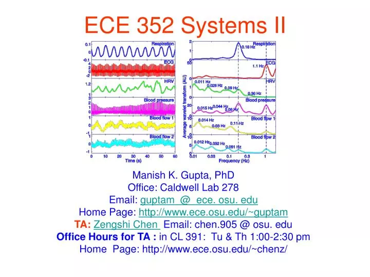
ECE 352 Systems II. Manish K. Gupta, PhD Office: Caldwell Lab 278 Email: guptam @ ece. osu. edu Home Page: http://www.ece.osu.edu/~guptam TA: Zengshi Chen Email: chen.905 @ osu. edu Office Hours for TA : in CL 391: Tu & Th 1:00-2:30 pm Home Page: http://www.ece.osu.edu/~chenz/.

E N D
ECE 352 Systems II Manish K. Gupta, PhD Office: Caldwell Lab 278 Email: guptam @ ece. osu. edu Home Page: http://www.ece.osu.edu/~guptam TA:Zengshi Chen Email: chen.905 @ osu. edu Office Hours for TA : in CL 391: Tu & Th 1:00-2:30 pm Home Page: http://www.ece.osu.edu/~chenz/
Acknowledgements • Various graphics used here has been taken from public resources instead of redrawing it. Thanks to those who have created it. • Thanks to Brian L. Evans and Mr. Dogu Arifler • Thanks to Randy Moses and Bradley Clymer
Slides edited from: • Prof. Brian L. Evans and Mr. Dogu Arifler Dept. of Electrical and Computer Engineering The University of Texas at Austin course: EE 313 Linear Systems and Signals Fall 2003
Z-transforms • For discrete-time systems, z-transforms play the same role of Laplace transforms do in continuous-time systems • As with the Laplace transform, we compute forward and inverse z-transforms by use of transforms pairs and properties Bilateral Forward z-transform Bilateral Inverse z-transform
Region of the complex z-plane for which forward z-transform converges Four possibilities (z=0 is a special case and may or may not be included) Im{z} Im{z} Entire plane Disk Re{z} Re{z} Im{z} Im{z} Intersection of a disk and complement of a disk Complement of a disk Re{z} Re{z} Region of Convergence
h[k] = d[k] Region of convergence: entire z-plane h[k] = d[k-1] Region of convergence: entire z-plane h[n-1] z-1 H(z) h[k] = ak u[k] Region of convergence: |z| > |a| which is the complement of a disk Z-transform Pairs
Stability • Rule #1: For a causal sequence, poles are inside the unit circle (applies to z-transform functions that are ratios of two polynomials) • Rule #2: More generally, unit circle is included in region of convergence. (In continuous-time, the imaginary axis would be in the region of convergence of the Laplace transform.) • This is stable if |a| < 1 by rule #1. • It is stable if |z| > 1 > |a| by rule #2.
Inverse z-transform • Yuk! Using the definition requires a contour integration in the complex z-plane. • Fortunately, we tend to be interested in only a few basic signals (pulse, step, etc.) • Virtually all of the signals we’ll see can be built up from these basic signals. • For these common signals, the z-transform pairs have been tabulated (see Tables)
Example • Ratio of polynomial z-domain functions • Divide through by the highest power of z • Factor denominator into first-order factors • Use partial fraction decomposition to get first-order terms
Example (con’t) • Find B0 by polynomial division • Express in terms of B0 • Solve for A1 and A2
Express X[z] in terms of B0, A1, and A2 Use table to obtain inverse z-transform With the unilateral z-transform, or the bilateral z-transform with region of convergence, the inverse z-transform is unique. Example (con’t)
Z-transform Properties • Linearity • Shifting
Z-transform Properties • Convolution definition • Take z-transform • Z-transform definition • Interchange summation • r = k - m • Z-transform definition
Linear Difference Equations • Discrete-timeLTI systemscan becharacterizedby differenceequations y[k] = (1/2) y[k-1] + (1/8) y[k-2] + f[k] • Taking z-transform of the difference equation gives description of the system in the z-domain + f[k] y[k] + UnitDelay + 1/2 y[k-1] UnitDelay 1/8 y[k-2]
Advances and Delays • Sometimes differential equations will be presented as unit advances rather than delays y[k+2] – 5 y[k+1] + 6 y[k] = 3 f[k+1] + 5 f[k] • One can make a substitution that reindexes the equation so that it is in terms of delays Substitute k with k-2 to yield y[k] – 5 y[k-1] + 6 y[k-2] = 3 f[k-1] + 5 f[k-2] • Before taking the z-transform, recognize that we work with time k 0 so u[k] is often implied y[k-1] = y[k-1] u[k] y[k-1] u[k-1]
Example • System described by a difference equation y[k] – 5 y[k-1] + 6 y[k-2] = 3 f[k-1] + 5 f[k-2] y[-1] = 11/6, y[-2] = 37/36 f[k] = 2-k u[k]
Transfer Functions • Previous example describes output in time domain for specific input and initial conditions • It is not a general solution, which motivates us to look at system transfer functions. • In order to derive the transfer function, one must separate • “Zero state” response of the system to a given input with zero initial conditions • “Zero input” response to initial conditions only
Transfer Functions • Consider the zero-state response • No initial conditions: y[-k] = 0 for all k > 0 • Only causal inputs: f[-k] = 0 for all k > 0 • Write general nth order difference equation
F[z] H[z] Y[z] Stability • Knowing H[z], we can compute the output given any input • Since H[z] is a ratio of two polynomials, the roots of the denominator polynomial (called poles) control where H[z] may blow up • H[z] can be represented as a series • Series converges when poles lie inside (not on) unit circle • Corresponds to magnitudes of all poles being less than 1 • System is said to be stable
Relation between h[k] and H[z] • Either can be used to describe the system • Having one is equivalent to having the other since they are a z-transform pair • By definition, the impulse response, h[k], is y[k] = h[k] when f[k] = d[k] Z{h[k]} = H[z] Z{d[k]} H[z] = H[z] · 1 h[k] H[z] • Since discrete-time signals can be built up from unit impulses, knowing the impulse response completely characterizes the LTI system
Complex Exponentials • Complex exponentials havespecial property when theyare input into LTI systems. • Output will be same complexexponential weighted by H[z] • When we specialize the z-domain to frequency domain, the magnitude of H[z] will control which frequencies are attenuated or passed.
Z and Laplace Transforms • Are complex-valued functions of a complex frequency variable Laplace: s = + j 2 f Z: z = ejW • Transform difference/differential equations into algebraic equations that are easier to solve
f[k] H[z] y[k] Z Laplace H[esT] Z and Laplace Transforms • No unique mapping from Z to Laplace domain or vice-versa • Mapping one complex domain to another is not unique • One possible mapping is impulse invariance. • The impulse response of a discrete-time LTI system is a sampled version of a continuous-time LTI system.
f[k] H[z] y[k] Z Laplace H[esT] Z and Laplace Transforms
Im{s} Im{z} 1 Re{s} Re{z} -1 1 1 -1 Impulse Invariance Mapping • Impulse invariance mapping is z = e s T s = -1 j z = 0.198 j 0.31 (T = 1) s = 1 j z = 1.469 j 2.287 (T = 1)
s(t) Ts t Sampling • Many signals originate as continuous-time signals, e.g. conventional music or voice. • By sampling a continuous-time signal at isolated, equally-spaced points in time, we obtain a sequence of numbers k {…, -2, -1, 0, 1, 2,…} Ts is the sampling period Sampled analog waveform
Shannon Sampling Theorem • A continuous-time signal x(t) with frequencies no higher than fmax can be reconstructed from its samples x[k] = x(k Ts) if the samples are taken at a rate fswhich is greater than 2 fmax. • Nyquist rate = 2 fmax • Nyquist frequency = fs/2. • What happens if fs = 2fmax? • Consider a sinusoid sin(2 p fmax t) • Use a sampling period of Ts = 1/fs = 1/2fmax. • Sketch: sinusoid with zeros at t = 0, 1/2fmax, 1/fmax, …
Sampling Theorem Assumptions • The continuous-time signal has no frequency content above the frequency fmax • The sampling time is exactly the same between any two samples • The sequence of numbers obtained by sampling is represented in exact precision • The conversion of the sequence of numbers to continuous-time is ideal
Why 44.1 kHz for Audio CDs? • Sound is audible in 20 Hz to 20 kHz range: fmax = 20 kHz and the Nyquist rate 2 fmax = 40 kHz • What is the extra 10% of the bandwidth used? Rolloff from passband to stopband in the magnitude response of the anti-aliasing filter • Okay, 44 kHz makes sense. Why 44.1 kHz? At the time the choice was made, only recorders capable of storing such high rates were VCRs. NTSC: 490 lines/frame, 3 samples/line, 30 frames/s = 44100 samples/s PAL: 588 lines/frame, 3 samples/line, 25 frames/s = 44100 samples/s
Sampling • As sampling rate increases, sampled waveform looks more and more like the original • Many applications (e.g. communication systems) care more about frequency content in the waveform and not its shape • Zero crossings: frequency content of a sinusoid • Distance between two zero crossings: one half period. • With the sampling theorem satisfied, sampled sinusoid crosses zero at the right times even though its waveform shape may be difficult to recognize
Analog sinusoid x(t) = A cos(2pf0t+ f) Sample at Ts = 1/fs x[k] = x(Ts k) =A cos(2p f0 Ts k + f) Keeping the sampling period same, sample y(t) = A cos(2p(f0 + lfs)t + f) where l is an integer y[k] = y(Ts k) = A cos(2p(f0 + lfs)Tsk + f) = A cos(2pf0Tsk + 2p lfsTsk + f) = A cos(2pf0Tsk + 2p l k + f) = A cos(2pf0Tsk + f) = x[k] Here, fsTs = 1 Since l is an integer,cos(x + 2pl) = cos(x) y[k] indistinguishable from x[k] Aliasing
Aliasing • Since l is any integer, an infinite number of sinusoids will give same sequence of samples • The frequencies f0 + l fs for l 0 are called aliases of frequency f0with respect fsto because all of the aliased frequencies appear to be the same as f0when sampled by fs
Generalized Sampling Theorem • Sampling rate must be greater than twice the bandwidth • Bandwidth is defined as non-zero extent of spectrum of continuous-time signal in positive frequencies • For lowpass signal with maximum frequency fmax, bandwidth is fmax • For a bandpass signal with frequency content on the interval [f1, f2], bandwidth is f2 - f1
Example: Second-Order Equation • y[k+2] - 0.6 y[k+1] - 0.16 y[k] = 5 f[k+2] withy[-1] = 0 and y[-2] = 6.25 and f[k] = 4-k u[k] • Zero-input response Characteristic polynomial g2 - 0.6 g - 0.16 = (g + 0.2) (g - 0.8) Characteristic equation (g + 0.2) (g - 0.8) = 0 Characteristic roots g1 = -0.2 and g2 = 0.8 Solution y0[k] = C1 (-0.2)k + C2 (0.8)k • Zero-state response
Example: Impulse Response • h[k+2] - 0.6 h[k+1] - 0.16 h[k] = 5 d[k+2]with h[-1] = h[-2] = 0 because of causality • In general, from Lathi (3.41), h[k] = (b0/a0) d[k] + y0[k] u[k] • Since a0 = -0.16 and b0 = 0, h[k] = y0[k] u[k] = [C1 (-0.2)k + C2 (0.8)k] u[k] • Lathi (3.41) is similar to Lathi (2.41): Lathi (3.41) balances impulsive events at origin
Example: Impulse Response • Need two values of h[k] to solve for C1 and C2 h[0] - 0.6 h[-1] - 0.16 h[-2] = 5 d[0] h[0] = 5 h[1] - 0.6 h[0] - 0.16 h[-1] = 5 d[1] h[1] = 3 • Solving for C1 and C2 h[0] = C1 + C2 = 5 h[1] = -0.2 C1 + 0.8 C2 = 3 Unique solution C1 = 1, C2 = 4 • h[k] = [(-0.2)k + 4 (0.8)k] u[k]
Example: Solution • Zero-state response solution (Lathi, Ex. 3.13) ys[k] = h[k] * f[k] = {[(-0.2)k + 4(0.8)k] u[k]} * (4-ku[k]) ys[k] = [-1.26 (4)-k + 0.444 (-0.2)k + 5.81 (0.8)k] u[k] • Total response: y[k] = y0[k] + ys[k] y[k] = [C1(-0.2)k + C2(0.8)k] + [-1.26 (4)-k + 0.444 (-0.2)k + 5.81 (0.8)k] u[k] • With y[-1] = 0 and y[-2] = 6.25 y[-1] = C1 (-5) + C2(1.25) = 0 y[-2] = C1(25) + C2(25/16) = 6.25 Solution: C1 = 0.2, C2 = 0.8
Repeated Roots • For r repeated roots of Q(g) = 0 y0[k] = (C1 + C2k + … + Crkr-1) gk • Similar to the continuous-time case
Im g Unstable Re g Marginally Stable g Stable |g| b -1 1 Lathi, Fig. 3.16 Stability for an LTID System • Asymptotically stable if andonly if all characteristic rootsare inside unit circle. • Unstable if and only if one orboth of these conditions exist: • At least one root outside unit circle • Repeated roots on unit circle • Marginally stable if and only if no roots are outside unit circle and no repeated roots are on unit circle (see Figs. 3.17 and 3.18 in Lathi)
Im g Im l Marginally Stable Marginally Stable Unstable Re g Re l -1 1 Stable Stable Unstable Stability in Both Domains Continuous-Time Systems Discrete-Time Systems Marginally stable: non-repeated characteristic roots on the unit circle (discrete-time systems) or imaginary axis (continuous-time systems)
Frequency Response • For continuous-time systems the response to sinusoids are • For discrete-time systems in z-domain • For discrete-time systems in discrete-time frequency
Response to Sampled Sinusoids • Start with a continuous-time sinusoid • Sample it every Tseconds (substitute t = k T) • We show discrete-time sinusoid with • Resulting in • Discrete-time frequency is equal to continuous-time frequency multiplied by sampling period
Example • Calculate the frequency response of the system given as a difference equation as • Assuming zero initial conditions we can take the z-transform of this difference equation • Since