Download

1 / 36
360 likes | 366 Views
Multi-Frequency Polarization Studies of AGN Jets Denise Gabuzda (University College Cork). Outline of talk — Image alignmnent/core shifts/core B fields Faraday rotation studies Investigations of image properties using Monte Carlo simulations. Image alignment, core shifts, core B fields.

E N D
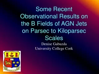
Multi-Frequency Polarization Studies of AGN JetsDenise Gabuzda (University College Cork)
Outline of talk — • Image alignmnent/core shifts/core B fields • Faraday rotation studies • Investigations of image properties using Monte Carlo simulations
Why image alignment is necessary Schematic from Kovalev et al. (2007) VLBI “core” = optically thick base of jet, moves further down jet at increasingly lower frequencies
VLBI images align on bright, compact cores rather than optically thin jet features, absolute position info lost, direct superposition yields erroneous spectral indices.
Alignment techniques • Based on comparing positions of optically thin features • Model fitting • Image cross-correlation analyses • In practice – different approaches work best for different source structures, but both can yield reliable alignments
Lobanov (1998): • Approach to estimating pc-scale B field strengths based on measurement of frequency-dependent position of VLBI core (Konigl 1981) • Few sources, few frequencies, but a start More recent studies: O’Sullivan & Gabuzda (2010) — only a few sources, but 8 frequencies (detailed, redundant information) Kovalev et al. (2009) — 29 sources, 2 frequencies Sokolovskii et al. (2011) — 20 sources, 9 frequencies Pushkarev et al. (2012) — more than a hundred well studied (MOJAVE) sources, four frequencies
O’Sullivan & Gabuzda 2010 2007+777 kr = [(3–2)m + 2n–2]/(5–2) B ~ r –m N ~ r –n r ~ –1/kr • Behaviour expected for Blandford–Konigl jet is observed • Evidence for equipartition in most cores – values for parameter kr often close to 1, suggests B ~ r –1 and N ~ r –2
O’Sullivan & Gabuzda 2010 • Inferred core-region B fields are tenths of Gauss • Data consistent with B ~ r –1 • Extrapolation of B field to smaller scales gives values consistent with magnetic launching of jets (points shown are for rg and 10rg; Komissarov et al. 2007)
Pushkarev et al. (2012) • Ability to compare shifts for different types of AGNs. • Shift distribution peaked in jet direction, as expected
Pushkarev et al. (2012) • B fields in quasars somewhat higher than in BL Lac objects
Faraday rotation – rotation of the observed linear polarisation angle when polarised EM wave passes through a magnetised plasma. = o + RM 2 RM = (constants) ne B•dl Electron density Line of sight B field
Zavala & Taylor (2003, 2004) • 40 objects • Core RM > Jet RM • Sometimes sign changes (changes in LOS B field) • Quasar core RMs > BL Lac core RMs
If jet has a helical B field, should observe a Faraday-rotation gradient across the jet – due to systematically changing line-of-sight component of B field across the jet (Blandford 1993). RM < 0 RM ~ ne B•dl B Jet axis RM > 0 Simulation by Broderick & McKinney 2010 •
Croke, O’Sullivan & Gabuzda 2010 Algaba 2012 Gabuzda et al. 2013 Hovatta et al. 2012 Reports of transverse RM gradients across pc-scale AGN jets, suggested as evidence for helical B fields
Is the field toroidal or helical on parsec scales? Murphy et al. (2013) Fitting asymmetric transverse pol profiles for Mrk501 using simple helical field model – yields consistent fits with pitch angle ~ 53°, viewing angle in jet rest frame ~ 83° (see Coughlan poster, #21) Note: Mrk501 also has RM grad (Gabuzda et al. 2004, Croke et al. 2010)
Coughlan poster (#21) – another example Asymmetric transverse pol structure revealed by high-res MEM pol map + Transverse RM gradient ===> Helical (not just toroidal) field present on pc scales
Murphy et al. (2013) Fitted value for viewing angle in jet rest frame ’ together with measurement of apparent speeds can give solution for intrinsic jet speed (Lorentz factor) and viewing angle in rest frame of observer : =====> Yields for Mrk501 =0.96 and = 15º, consistent with results of Giroletti et al. (2004), ≥ 0.88 and ≤ 27º
Mahmud et al. (2012) Reversals of the transverse RM gradient between core region and jet on parsec scales in two AGNs Jet direction 4.6, 5, 7.9, 8.4, 12.9, 15.4 GHz 1.35, 1.43, 1.49, 1,67 GHz
Can be explained if “outgoing” B field in jet/inner accretion disc closes in outer disc Winding up of field lines due to differential rotation Integration path passes through both regions of helical field neB•dl Provides direct evidence for the presence of a “return field” in a more extended region surrounding the jet
Christodoulou et al. (in prep), Gabuzda et al. (2012) – finding some transverse RM gradients on kpc scales in literature Fewer kpc-scale than pc-scale jets show transverse RM gradients — may reflect different relative contributions from systematic (helical/toroidal) and random (turbulent) RM components on different scales (also talk by J. C. Algaba) Bonafede et al. 2010
How well resolved must the jets be to detect transverse RM gradients associated with helical B fields? • Transverse RM gradient visible in theoretical simulations of Broderick & McKinney (2010), even with a 1-mas beam • Spurious non-monotonicity possible in core region for some viewing angles, but observed direction of RM gradient is usually correct • Suggests we should be able to observe this effect Broderick & McKinney 2010
Taylor & Zavala (2010) proposed 4 criteria for transverse RM gradients to be reliable: • Criteria 2, 3, 4 have been applied in most previous studies anyway, do not add anything new • Criterion 1 was presented without justification, but would reject nearly all reported RM-gradient detections • Situation needed to be clarified!
Hovatta et al. (2012) • MC simulations to investigate statistical occurrence of spurious RM gradients due to noise and limited baseline coverage for 7.9, 8.4, 12.9, 15.4 GHz VLBA data • Fewer than ~1% of runs gave spurious 3 gradients, even for observed jet widths ~1.5 beam widths • Few spurious 2 gradients, too, but number can exceed 5% for widths below ~ 2 beam widths
Results confirmed by Murphy poster (#12):1.36, 1.43, 1.49, 1.67 GHz Algaba (2012):12, 15, 22 GHz 1 ——2 ——3 —— Behaviour very similar, details depend on frequency range considered. In all cases, show that the “3 beamwidth” criterion of Taylor & Zavala (2010) is too severe.
Mahmud et al. (2013):4.6, 5, 7.9, 8.4, 12.9, 15.4 GHz • Monte Carlo studies of simulated maps with transverse RM gradients for various intrinsic jet widths With realistic noise and baseline coverage, simulated RM gradients clearly visible even when jet width << beam width! Jet width 1/5 beam Jet width 1/3 beam Jet width 1/20 beam Jet width 1/10 beam
Murphy poster (#12): 1.36, 1.43, 1.49, 1.67 GHz Jet width 0.05 beam Jet width 0.40 beam 98% or more of simulated maps showed transverse RM gradients > 3 when intrinsic jet width was at least 1/5 of a beam width.
Summary - Core shifts, core B fields • Variety of image–alignment techniques have been developed and are being actively used • Core shift/core B-field studies carried out for large numbers of frequencies and large source samples for the first time • Most results consistent with equipartition in core region • 15-GHz core B fields range from ~ 0.02 G – 0.8 G • Data consistent with B ~ r –1 • Core B fields somewhat lower in BL Lac objects than in quasars
Summary – Faraday Rotation • Core RMs > Jet RMs (high electron density and B fields) • Core RMs lower in BL Lacs than in quasars • Transverse RM gradients (and transverse pol structure, EVPA rotations) provide direct evidence for helical/toroidal jet B fields, naturally formed by rotation of central BH + jet outflow. — Jets are fundamentally EM structures, launching mechanism also probably EM — Jets carry current – implications for collimation • Evidence for return field in region surrounding the jet
Summary – Monte Carlo Simulations • “3 beam width” criterion of Taylor & Zavala (2010) for reliability of transverse RM gradients is too severe • Best criteria for reliability are RM difference ( > 3) and monotonicity • Transverse RM gradients in simulated images can be visible even when intrinsic jet width is << beam width • Note: need less resolution to detect presence of gradients than to reliably derive source parameters! • Usual practice of assigning I, Q or U errors to be equal to rms appreciably underestimates uncertainties (by about a factor of 2 off peak) (Hovatta et al. 2012)
Key future “technical” work: • Improve understanding of uncertainties in fluxes measured in individual pixels • Mathematical description of correlations between fluxes measured in nearby pixels • Development of alternative imaging techniques for VLBI (e.g. MEM, RM synthesis)
A cat who is has found something far more interesting than multi-frequency polarization measurements.
4/1997 6/2000 Trans RM gradient in 1803+784 changed direction with time (Mahmud et al. 2009)! 8/2002 8/2003