Download
1 / 52
530 likes | 608 Views
CSE 554 Lecture 8: Laplacian Deformation. Fall 2012. Review. Source. Alignment Registering source to target by rotation and translation Rigid-body transformations Methods Aligning principle directions (PCA) Aligning corresponding points (SVD) Iterative improvement (ICP)

E N D
CSE 554Lecture 8: Laplacian Deformation Fall 2012
Review Source • Alignment • Registering source to target by rotation and translation • Rigid-body transformations • Methods • Aligning principle directions (PCA) • Aligning corresponding points (SVD) • Iterative improvement (ICP) • Combines PCA and SVD Input Target After PCA After ICP
Non-rigid Registration • Rigid alignment cannot account for shape variance • Non-rigid deformation can give a better fit Source Target Rigid alignment After non-rigid deformation
Non-rigid Registration • A minimization problem • Minimizing the distance between the deformed source and the target • “Fitting term” • Minimizing the distortion to the source shape • “Distortion term”
Intrinsic vs. Extrinsic • Intrinsic methods • Deforms points on the source curve/surface • App: boundary curve or surface matching • Extrinsic methods • Deforms all points on and interior to the source curve/surface • App: image or volume matching
Laplacian-based Deformation • An intrinsic method • Simple, efficient, producing reasonable results • Preserving local shape features • Widely used in graphics applications for interactive deformation • Reference: “Laplacian surface editing”, by Sorkine et al., 2004 (citation ~ 500)
Setup • Input • Source with n points: p1,…,pn • Let the first m points be “handles” • Target location of handles: q1,…,qm • Output • Deformed locations of source points: p1’,…,pn’ When deforming the source to fit a target shape: m=n and qi is the point on the target closest to pi. Deformed Source q2 p3=q3 p1=q1 p2 An example with 3 target points, two of which are stationary (red)
Overview • Finding deformed locations pi’ that minimize: • Ef: fitting term • Measures how close are the deformed source to the target • Ed: distortion term • Measures how much the source shape is changed
Fitting Term • Sum of squared distances to target handle locations q2 p2
Distortion Term • Q: How to measure shape? • A: By “bumpiness” at each vertex • Laplacian: vector from the centroid of neighbors to the vertex • Recall that in fairing, we reduced this vector to “smooth out” bumps • A linear operator over point locations where Ni are indices of neighboring vertices of pi
Distortion Term • Minimizing changes in Laplacians during deformation • Over all source points i: Laplacian at pi before deformation
Putting Together • Finding deformed locations pi’ that minimize: • A quadratic equation in terms of variables (pix’, piy’, piz’) • qi, i are constants • L[] is a linear operator
Quadratic Minimization • A general form of quadratic minimization: • There are s variables: x=(x1,…,xs)T • Each a1,…, ak is a length-s column vector (linear coefficients) • Each b1,…, bk is a scalar (constant coefficients) • k should be greater than s (so that the problem is over-constrained)
Quadratic Minimization • To solve: • Re-write in matrix form: where is a k by s matrix is a length-k vector
Quadratic Minimization • The minimizer is where the partial derivatives are all zero • To solve for x in this equation: • Taking matrix inverse (good for small s, but numerically unstable for large s) • Using specialized linear system solver (LinearSolve in Mathematica, TNT/LAPACK in C)
Quadratic Minimization • Re-writing our minimization in the general form • In 2D, there are 2n variables: x = (p1x’,…, pnx’, p1y’,…, pny’ )T • In 3D, there are 3n variables • We will next re-write each quadratic term in 2D as (aix-bi)2 • Can be extended easily to 3D
Quadratic Minimization • The ai and bi in the fitting term • There are 2m quadratic terms • In the first set of m terms: • For i=1,…,m, bi=qix, ai contains all zero, except its (i)th entry is 1. • In the second set of m terms: • For i=1,…,m, bi+m=qiy, ai+m contains all zero, except its (i+n)th entry is 1
Quadratic Minimization • The ai and bi in the fitting term • There are 2m quadratic terms • Example with 3 vertices and 2 fitting constraints (n=3; m=2):
Quadratic Minimization • The ai and bi in the distortion term: • There are 2n quadratic terms • The first set of n terms: • For i=1,…,n, ai is all zero except the (i)th entry is 1, the (j)th entries are -1/|Ni| for all jNi, and bi=ix • The second set of n terms: • For i=1,…,n, ai+n is all zero except the (i+n)th entry is 1, the (j+n)th entries are -1/|Ni| for all jNi, and bi+n=iy
Quadratic Minimization • The ai and bi in the distortion term: • There are 2n quadratic terms • Example with 3 vertices (n=3):
Summary • Compute Laplacians (i) • Construct coefficients (ai, bi) • Stick them into matrices (A,B) • Solve (x)
Results Deformed A small deformation
Results Deformed A larger deformation
Results Deformed Stretching
Results Deformed Shrinking
Results Deformed Rotation
Discussion • Limitations • Local features are “skewed”, and they don’t scale with the model • Reason: Laplacian changes with rotation or scale • Two bumps that differ by rotation or scale have different Laplacians • Which will be penalized by our distortion term
A Better Distortion Term • Not penalizing rotation and scaling of local features • Transforming the original Laplacian vectors before comparing to the deformed Laplacians • Tiis a matrix that describes how the local shape around pi is deformed
Key Questions • How to represent transformations as matrices? • How to compute Ti? • We will focus in the derivations of the 2D case • 3D results will be briefly presented at the end
Transformation Matrices (2D) • Homogeneous coordinates • A 2D point: (x,y,1) • A 2D vector: (x,y,0) • A 3D point: (x,y,z,1) • A 3D vector: (x,y,z,0)
Transformation Matrices (2D) • Translation • Cartesian coordinates: vector addition • Homogeneous coordinates: matrix product
Transformation Matrices (2D) • Isotropic scaling • Cartesian coordinates: vector scaling • Homogeneous coordinates: matrix product
Transformation Matrices (2D) • Rotation • Cartesian coordinates: matrix product • Homogeneous coordinates: matrix product
Transformation Matrices (2D) • Summary of elementary similarity transformations • To combine transformations: take the product of these matrices Translation by vector v Scaling by scalar s Rotation by angle
Similarity Transforms (2D) • General similarity transformations • The product of any set of elementary matrices can be written this way • Any choice of (a, w, tx, ty) can be written as a sequence of rotation, isotropic scaling and translation • Note that a and w can’t be both zero
Computing Ti (2D) • Suppose we know the deformed locations pi’ • Compute Ti as the similarity transform that best fits the neighborhood of pi to that of pi’
Computing Ti (2D) • Suppose we know the deformed locations pi’ • Compute Ti as the similarity transform that best fits the neighborhood of pi to that of pi’ • This is a quadratic minimization problem for entries of Ti • E.g., a, w, tx, ty
Computing Ti (2D) • The matrix form of the minimization is: where is a 2|Ni|+2 by 4 matrix, and Ni={i1, i2,…} are indices of neighboring vertices of pi
Computing Ti (2D) • By quadratic minimization: • Linear expressions of variables (pix’ , piy’)
Distortion Term (2D) • Two parts of each distortion term: • Transformed Laplacian: • Laplacian of the deformed locations: where where is a 2 by 2|Ni|+2 matrix
Distortion Term (2D) • Putting together: • They form 2n quadratic terms (aix-bi)2 for x = (p1x’,…, pnx’, p1y’,…, pny’ )T • All bi are zero • Each ai can be extracted from H where and are its rows
Results (2D) Old distortion term New distortion term
Results (2D) New distortion term Old distortion term
Results (2D) Old distortion term New distortion term
Results (2D) Old distortion term New distortion term
Registration • Use nearest neighbors as corresponding target locations • Assuming the source is already close to the target • Iterative closest point (ICP) • 1. For each point on the source, assign its closest point on the target as its corresponding point. Compute Laplacian-based deformation. • A threshold on the closest distance can be used to throw away unlikely correspondences • 2. Repeat step (1) until a termination criteria is met. • Maximum iteration or minimum RMSD improvement
Result After rigid alignment 1 iteration of Laplacian 7 iterations of Laplacian Overlaying all curves
Result • Weighting the distortion term large w medium w small w
Similarity Transforms (3D) • Elementary transformation matrices • To perform a sequence of transformations: take the product of these matrices Translation by vector v Scaling by scalar s Rotation by angle around X axis
Similarity Transforms (3D) • General similarity transformations in 3D • Approximates the product of a set of elementary matrices • Up to a small rotation angle • May introduce skewing for large rotations