Download
1 / 19
190 likes | 305 Views
Relative Efficiency of Government Spending and Its Determinants: Evidence from East Asian Countries. Eric C. Wang N ational Chung Cheng University, Taiwan Eskander Alvi W estern Michigan University, U.S.A. E urasian Economic Review, Spring 2011, 1(1) Economics, CCU 03-2011. Motivation

E N D
Relative Efficiency of Government Spending and Its Determinants:Evidence from East Asian Countries Eric C. Wang National Chung Cheng University, Taiwan Eskander Alvi Western Michigan University, U.S.A. Eurasian Economic Review, Spring 2011, 1(1) Economics, CCU 03-2011
Motivation In 2008 and 2009, a severe world-wide economic recession was experienced. Many countries adopted the government expenditure approach to stimulate the economy and to raise GDP. C-voucher-2009.doc Interesting remarks If different governments spend same amount of incremental expenditure (ΔG), will they create same amount of increase in GDP (ΔGDP)? Do governments perform equally well in managing their public expenditure?
Initiative Concepts Two major variables that will brings about differences in the performance of government expenditure among countries. 1. Government expenditure multiplier: mpc, mpi, mpm, marginal tax rate. 2. Macro-management ability of the government.
Purposes • To measure the relative performance of government spending of 7 Asian countries. • To investigate the factors that could influence government performance. • Japan, Singapore, Taiwan, Hong Kong, • Malaysia, Thailand, and Korea. • 1986 - 2007. • Data Envelopment Analysis (DEA) • Extreme Bounds Analysis (EBA) • associated with Truncated Tobit regression
Theoretical Background GDP = Y = C + I + G + (X-M) ΔY = ΔC +ΔI +ΔG +Δ(X-M) mG = ΔY /ΔG = 1/ [1-(mpc+mpi)(1-t)] mG varies from country to country, from time to time. Concept of production In the short-run, mG is beyond government control. Government is to choose an amount of ΔG to reach its goal of increase in GDP. ΔY can be generated by government spending ΔG and multiplier mG . In the long-run, a trade-off between ΔG and mG is possible.
Empirical Background DEA method Farrell’s (1957) Charnes, Cooper, and Rhodes (1978): CRTS Banker, Charnes, and Cooper (1984): VRTS ∆G /∆GDP P R Q 0 mG /∆GDP
DEA method applied in government sector: Lovell, et al. (1995):output-oriented DEA, policies on real GDP per capita, inflation, employment, trade balance of 19 OECD. Yaisawarng (2002):a DEA scheme assess the efficiency of government divisions; allocate budget according to efficiency. Leightner (2002):output-oriented DEA, government spending and GDP of 24 Asian countries. Rayp and Van De Sijpe (2007):efficiency of government expenditure in improving health, education, governance of 52 LDCs.
Hypotheses (I).Private sector’s activities will affect government’s performance in raising GDP. ΔGDP = ΔC +ΔI +ΔG +Δ(X-M) Besides ΔG, ΔGDP also depends on private sector’s activities, i.e. ΔC, ΔI, and Δ(X-M). [ΔC +ΔI +Δ(X-M)] / ΔGDP (II). Government corruption hypothesis. Bardhan, (1997); Treisman, (2000); Barreto (2000); Bose, et al., (2008); Grigor’ev and Ovchinnikov (2009) Corruption Perception Index (CPI):Transparency International
Hypotheses (III). Relationship between monetary expansion and government spending on promoting growth. Marini and van der Ploeg (1988); Dernburg (1992); Faria (2000); Kandil and Mirzaie (2006); Setterfield (2009). M1 and M2 growth rates (IV). Government size. Barro (1991); Hansson and Henrekson (1994); Folster and Henrekson (2001);Easterly and Rebelo (1993); Barro (1990); Kolluri and Wahab (2007). Government revenue / GDP Total Taxes / GDP
Quantitative Methods DEA Method DEA: a non-parametric model to distinguish between efficient and inefficient institutions. Minimize , z, subject to Y z yk , X z xk , I z = 1, z R+K . yk , xk:the output and input vectors for DMU k, z:a vector of weights, :a scalar value a proportional contraction of all inputs, The LP problem is solved K times.
EBA Method with Tobit Regression Truncated Tobit Model A regression model designed for data with censored nature. Left-censored Right-censored Censored at both ends Efficiency score in the range of 0 and 1
IEj,k* = f j ( Qj,k ; j , j uj,k ) j = 1, …, N (countries)k = 1, …, K (years) Properties: IEj,k= IEj,k* if IEj,k* > 0 IEj,k = 0 if IEj,k* 0 IEj,k:country j’s observed inefficiency scores for year k based on DEA results, IEj,k*:latent score value, Qj,k:vector of r factors influencing government efficiency for country j in year k, j:vector of coefficients, j :a parameter to be estimated, uj,k:disturbance term.
Extreme-Bounds-Analysis (EBA) Leamer (1983, 1985); Levine and Renelt (1992), etc. Core: Varying the subset of control variables included in the regression to find the widest range of coefficient estimates on the variables of interest that standard hypothesis tests do not reject. W = iI + mM + zZ +u W:the inefficiency scores I: always included variables M:variables of primary interest Z: a subset of macro-variables
Extreme Bound: The group of Z-variables that produces the maximum (minimum) value of m, plus two standard errors. Upper bound, Lower bound (1) If mremains significant and has the same sign within the extreme bounds, the result is referred to as “robust”. (2) If the coefficient does not remain significant or if the coefficient changes sign, then the result is seen as “fragile”.
Major Z-variables GDP per capita: Levine and Renelt, 1992; Saleh and Harvie, 2005 Secondary school enrollment rate: Mankiw et al. 1992; Barro, 1991 Unemployment rate: Young and Pedregal, 1999 Changes in GDP deflator: Neyapti, 2003 Interest rate: Cebula, 2003 Private credit / GDP Liquid liability / GDP ratio: Polokangas, 1993 Saving rate: Evans and Karras, 1996 Government debt / GDP: Saleh and Harvie, 2005 Non-Agricultural share in GDP
Data and Empirical Results Data: 7 countries, 1986-2007, Table 1. Estimation on Relative Efficiency Scores Since ΔG has both short-term & long-term effects on ΔGDP, we use ΔGDPt+1, ΔGDPt+2, and ΔGDPt+3 as outputs. Table 2
Preliminary Tobit Regression Δ(C+I+X-M)/ΔGDP as the I-variable The effect of recession on government performance is included. Table 3: 4 Tobit regressions The coefficients of the term Δ(C+I+X-M)/ΔGDP significantly negative. Corruption Perception Index (CPI) significantly negative. M2 growth rate holds a more significantly positive relationship . Table 4 identical regressors plus country-dummy variables. Table 5 using all I, M and Z-variables.
Robustness Tests using EBA Method • Table 6. • Robust • Δ(C+I+X-M)/ΔGDP significantly negative. 2. Corruption Perception Index (CPI) significantly negative. 3. M2 growth rate significantly positive. Fragile 1. M1 growth rate. 2. Government Revenue / GDP. 3. Government Taxes /GDP.