Download
1 / 16
160 likes | 433 Views
EE 313 Linear Systems and Signals Fall 2010. Signals. Prof. Brian L. Evans Dept. of Electrical and Computer Engineering The University of Texas at Austin. Initial conversion of content to PowerPoint by Dr. Wade C. Schwartzkopf. Course Outline. Roberts, ch. 1-3.

E N D
EE 313 Linear Systems and Signals Fall 2010 Signals Prof. Brian L. Evans Dept. of Electrical and Computer Engineering The University of Texas at Austin Initial conversion of content to PowerPointby Dr. Wade C. Schwartzkopf
Course Outline Roberts, ch. 1-3 • Time domain analysis (lectures 1-10) Signals and systems in continuous and discrete time Convolution: finding system response in time domain • Frequency domain analysis (lectures 11-16) Fourier series Fourier transforms Frequency responses of systems • Generalized frequency domain analysis (lectures 17-26) Laplace and z transforms of signals Tests for system stability Transfer functions of linear time-invariant systems Roberts, ch. 4-7 Roberts, ch. 9-12
Signals • A function, e.g. sin(t) in continuous-time orsin(2 p n / 10) in discrete-time, useful inanalysis • A sequence of numbers, e.g. {1,2,3,2,1} which is a sampled triangle function, useful insimulation • A collection of properties, e.g. evensymmetric about origin, useful inreasoningabout behavior • A piecewise representation, e.g. • A functional, e.g. the Diracdelta functional d(t)
Exponential Signals • Solutions to linear constant-coefficient differential equations, and hence, very common e-t et t t t = -1 : 0.01 : 1; e1 = exp(t); plot(t, e1) t = -1 : 0.01 : 1; e2 = exp(-t); plot(t, e2)
Exponential Signal Properties • Real-valued exponential signals Amplitude values are always non-negative Might decay or not as t goes to infinity • Complex-valued exponential signals We’ll need these properties throughout the semester
Piecewise Functions • Unit area rectangular pulse • What does rect(x / a) look like? • Unit triangle function rect(t) 1 t -1/2 0 1/2 Math commands rectpuls(t) tripuls(0.5*t) tri(t) 1 t -1 0 1 Both functions are even symmetric about origin.
-e e t -e e t Dirac Delta Functional • Mathematical idealism foran instantaneous event • Dirac delta as generalizedfunction (a.k.a. functional) Unit area: Sifting provided g(t) is defined at t = 0 Scaling: • Note that d(0) is undefined Unit Area Unit Area
(1) Unit Area t 0 Dirac Delta Functional • Generalized sifting, assuming that a > 0 • By convention, plot Dirac delta as arrow at origin Undefined amplitude at origin Denote area at origin as (area) Height of arrow is irrelevant Direction of arrow indicates sign of area • Simplify Dirac delta terms only under integration
We can simplify d(t) under integration What about? Answer: 0 What about? By substitution of variables, Other examples What about at origin? Dirac Delta Functional Before Impulse After Impulse
Unit Step Function • Models event that turns on and stays on • Definition • What happens at the origin for u(t)? u(0-) = 0 and u(0+) = 1, but u(0) can take any value Textbook uses u(0) = ½ to average left and right hand limits Impulse invariance filter design uses u(0) = ½ L. B. Jackson, “A correction to impulse invariance,” IEEE Signal Processing Letters, vol. 7, no. 10, Oct. 2000, pp. 273-275. Math command stepfun(t,0) defines u(0) = 1
Ramp ramp(t) = tu(t) Unit comb Impulse train Other Important Functions (1) (1) (1) (1) (1) (1) t t -2 -1 0 1 2 3 t = -3 : 0.01 : 3; r = t .* stepfun(t,0); plot(t, r)
Even symmetric about origin • Zero crossings at • Amplitude decreases proportionally to 1/t Sinc Function t = -5 : 0.01 : 5; s = sinc(t); plot(t, s)
Sampling • Many signals originate as continuous-time signals, e.g. voice or conventional music • Sample continuous-time signal at equally-spaced points in time to obtain discrete-time signal y[n] = y(nTs) n {…, -2, -1, 0, 1, 2,…} Ts is sampling period • Example Ts 3 4 5 6 7 n 1 2 y(t)
Audio CD Samples at 44.1 kHz • Human hearing is from about 20 Hz to 20 kHz • Sampling theorem (covered at mid-semester): sample continuous-time signal at rate of more than twice highest frequency in signal • Analog-to-digital conversion for audio CD First, apply a filter to pass frequencies up to 20 kHz (called a lowpass filter) and reject high frequencies. Lowpass filter needs 10% of cutoff frequency to roll off to zero (filter can reject frequencies above 22 kHz) Second, sample at 44.1 kHz captures analog frequencies of up to but not including 22.05 kHz Third, quantize to 16 bits per sample
d[n] 1 n -2 -1 0 1 2 3 u[n] 1 n -2 -1 0 1 2 3 Discrete-Time Impulse and Step • Impulse function Also called Kronecker Delta Even symmetric about origin • Unit step (unit sequence) n = -2 : 3; u = stepfun(n,0); stem(n, u);
Sinusoidal signal in continuous time Sample using sampling period Ts Substitute Ts= 1 / fs, fs is sampling rate, Discrete-time frequency Given integers N and L with common factors removed, discrete-timesinusoid hasperiod L if Example: singing a tone during cell phone call Discrete-Time Sinusoidal Signals