Download
1 / 54
540 likes | 694 Views
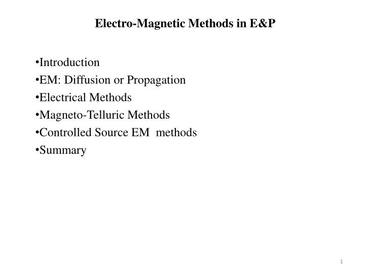
Electro-Magnetic Methods in E&P. Introduction EM: Diffusion or Propagation Electrical Methods Magneto-Telluric Methods Controlled Source EM methods Summary. Jaap C. Mondt. 1953-1959: Primary school 's-Gravenzande 1959-1964: Secondary school (HBS) 's-Gravenhage

E N D
Electro-Magnetic Methods in E&P Introduction EM: Diffusion or Propagation Electrical Methods Magneto-Telluric Methods Controlled Source EM methods Summary
Jaap C. Mondt 1953-1959: Primary school 's-Gravenzande 1959-1964: Secondary school (HBS) 's-Gravenhage 1964-1965: Lakeview High School, Battle Creek, USA 1965-1968: University Leiden: Bachelors Geology 1968-1972: University Utrecht: Masters Geophysics 1972-1977: University Utrecht: Ph.D. “Full wave theory and the structure of the lower mantle” 1977-1982: Shell Research: Interpretation Research on lithology and fluid prediction. 1982-1985: Shell Expro, Londen: Interpretation Central Northsea area acquisition and interpretation of Vertical Seismic Profiles 1985-1988: Shell Research: Seismic Data processing, evaluation of new processing methods for land and marine data. 1988-1991: Shell Research: Interpretation methods, development of interactive workstation methods 1991- 1995: SIPM: Evaluation of Contractor Seismic data processing 1995-2001: Shell Learning Centre Noordwijkerhout: Course Director Geophysics 2001-2007: SIEP: Potential Field Methods 2007- Geophysical Consultant (Breakaway, EPTS) Courses on Geophysical Data Acquisition, Processing and Interpretation
Q: Is electromagnenetics wave propagation or diffusion? • A: Wave propagation always involves attenuation & dispersion • Seismic waves • Diffusion = Wave propagation with (severe) attenuation • Perfume escaping from a bottle Introduction Electromagnetism A: EM can be considered to be wave propagation as well as diffusion. For high frequencies it has all the characteristics of wave propagation, For low frequencies it behaves more like diffusion Q: Source is a electrical dipole. When is it an electromagnetic source? A: When it is time varying, namely a time varying electric field will generate a magnetic field, hence the name electro-magnetic.
Resolution for Waves, Diffusion and Potential fields Seismic waves EM waves Resolution Time Derivatives Gravity
Electromagnetics: Propagation or Diffusion ? • early time • Intermediate • late time O Q: What will be observed over time at A with the source at the origin O? A: Particle density will increase and then decrease again, this will give the impression of a passing wave with an arrival time.
Diffusion: Skin depth / Wavelength The skin depth, d, is the distance over which the field strength is reduced by the factor 1/e = 0.368 ~-8.686 dB (m) The wavelength is (m) where r is the resistivity in W-m and f is the freq in Hz
Skin Depth/Wavelength for sea water, shales and reservoir 0.25 Hz 1 Hz Sea water resistivity 0.3 Ohm-m 0.3 Ohm-m skin depth 300 m 600 m wave length 1,886 m 3,771 m Shale resistivity 1.0 Ohm-m 1.0 Ohm-m skin depth 900 m 1,800 m wave length 5,657 m 11, 314 m HC filled reservoir 50.0 Ohm-m 50.0 Ohm-m skin depth 3,500 m 1,800 m wave length 22,000 m 44, 000 m
Electrical Monopole Current flow from a single surface electrode Current density: i=I/(2πr²) Am-2 Potential gradient: δV/δr=-ρi=- ρi/(2πr²) Vm-1
Rock resistivity SI unit of resistivity : ohm-metre (Ωm) Reciprocal of resistivity is conductivity : Siemens/metre (S/m)
Fractional Current The fraction of current penetrating below a depth Z for a current electrode separation L. Hence, 50% penetrates below L/Z=2 (Z=½L)
Apparent resistivity The variation of apparent resistivity with electrode separation over a single horizontal interface between media with increasing resistivities with depth.
Variation of apparent resistivity as a function of electrode separation for various resitivity sequences a b c a: At large enough electrode separation the apparent resistivity will equal the true resistivity. b: The intermediate higher/lower resistivity will appear at intermediate electrode separation. c: The deeper the higher/lower resistivity the larger the electrode separation (a) needed to observe its value.
Summary • Currents flow through the whole subsurface between electrodes. • 50% of the current flows in the subsurface above/below half the electrode spacing. • Commonly used field layouts: Wenner and Schlumberger configuration. • Wenner configuration: simpler (same spacing current and potential electrodes). • T here is “some” depth discrimination in the observed apparent resistivity. • True Inversion is needed to obtain better depth / spatial discrimination.
Source: Solar flares – 27 day cycle – main source of geomagnetic variations
Source: LightningMain energy source at frequencies above 1Hz. EARTH Schumann resonances at 8, 14, and 21 Hz.
Typical magnetic spectrum 5pT pT= pico Tesla
Time varying magnetic field Wave-front of time-varying magnetic fields Induced electric field Time-varying magnetic fields induce electric fields in the earth. The amplitudes of these are proportional to the resistivity.
Depth of penetration Skin depth: depth at which incident magnetic field is attenuated to 1/e of its orginal value Skin depth in metres = 500 SQRT(ρ/f) With ρ is resistivity of earth f is measurement frequency. Hence, by varying frequency, we vary the depth of penetration.
MT versus CSEM In MT the subsurface is derived from the relationship between the measured electric and magnetic data. This relationship is given by the (complex) transfer function called impedance tensor (Z) with elements: Zxy= Ex/Hy. The MT transfer function Z relates the horizontal electric field components Ex and Ey to the magnetic field components Hx and Hy .The vertical magnetic component Hz is related to the horizontal magnetic components via the Tipper vector: Hz = (A)Tx Hx + (B)Ty Hy and is only present in case of 3D structure (hence only 3D structures lifts the magnetic vector out of the horizontal plane, tips the vector up or down. MT is an inductive method and senses conductivity in the subsurface.
Typical lay-out in the field electrode Acquisition & processing unit Ey Battery Ex electrode Hx Common electrode electrode Hy Computer Hz electrode Magnetic sensors • H=magnetic field component • E=electric field component
E and H time series. Time Channels (top to bottom) are Ex,Ey, Hx, Hy, and Hz. Total Segment duration=1024 secs.
E and H components Time series are processed to give spectral estimates of the measured parameters, i.e. 2 electric and 3 magnetic fields at each site. These are denominated Ex Ey Hx Hy Hz E= electric and H=magnetic; x,y,z refer to the measurement axes.
Impedances calculated from the measured components Spectra are combined to give impedances (Zij), thus Zxy=Ex/Hy and so on. Since Ex etc are complex numbers, it follows that the impedances are also complex. In other words, they have an amplitude and a phase. The full MT site therefore has 4 horizontal impedance elements (Zxy, Zyx, Zxx, and Zyy), and also two vertical magnetic ones (Tzx and Tzy).
TE &TM Strike Ex TE Hy TE Hz Strike TM Strike Hx TM Ey Ez Traditionally the 2D sections were chosen in the dip direction. Hence, the TE has an E vector parallel to strike, whereas TM has an E vector in the dip direction, which crosses the structure and is more sensitive to its resistivity. Namely, the currents can’t go around the resistivity, whereas in TE they could. Hence, TM mode will show hydrocarbons in a traditional 2D acquisition.
Impedance matrix The horizontal components can be written as a tensor These are decomposed into 2 apparent resistivities and phases The general relationship is
Decomposition The most usual decomposition technique is to compute the parameters in the directions in which they are at their maximum and minimum for each relevant frequency. (Principal Axis Rotation) =TE in case of 2D geology = TM in case of 2D geology apparent resistivity phase Increasing period increasing depth
Impedance Polarisation The same data can be plotted as impedance polarization ellipses for each frequency: N Zxx Zxy These show the azimuthal variation of Z (hence resistivity). Here, the minimum apparent resistivity is N-S (parallel to strike) and the maximum is E-W.
1D sounding 1D 2D Libya NC171-5 Inverted to give resistivity versus depth
Example 2D sounding 1D 2D 1D 2D INVERTED TO GIVE RESISTIVITY v. DEPTH X-SECTION
Pseudo sections PERIOD APPARENT RESISTIVITY PERIOD PHASE DISTANCE ALONG PROFILE
Pseudo sections Res TE mode E parallel strike Phase Res TM mode E perp. strike Phase
Summary Magneto-Telluric • Passive method: using a natural source (solar activity, lighting) • Given the low “propagation”velocity in the subsurface the EM source-waves travel vertical downwards. • The frequency is low and hence the skin-depth very large. • In the field only receiver equipment is needed. • Is used as an early exploration tool (basin detection) • As it detects resistivity/conductivity it is used for mapping basement
Marine EM CSEM: Controlled Source EM Or Sea Bed Logging
CSEM: Sea Bed Logging Note: energy diffused through the air, seawater and subsurface
Source and Receivers EM receivers dropped at sea bottom EM Source towed above receivers
What is recorded at different offsets? Air waves DOMINATING WAVES Guided waves in the reservoir Air waves Direct waves HC Source-receiver distance
Troll: Off structure reference receiver Reservoir contour Towline 0 Offset NE Reference receiver Note: the receiver and source are both not above the the hydrocarbons 0 SW Offset NE
Troll: On structure versus Off structure receivers Reservoir contour Towline Normalize by reference receiver Reference receiver Now the source is above the hydrocarns
Troll: Depth estimate from Phase plot Reservoir contour Towline 0 Reference receiver SW Offset NE ½ offset at split = depth BML of anomaly Note the source is SW (not above the hydrocarbons) and NE of the receiver
Troll: Normalised magnitude at specific offset 2,5 Towline 2,0 Reservoir contour 1,5 Normalised Magnitude 1,0 0,5 0,0 0 -2000 -4000 -6000 -8000 -10000 -12000 Offset (m)
Troll (Gather Plot) Magnitude and seismic Maximum Anomaly Positions
Imaging Well-1 Well-2
Gather-plot (0.25Hz) Median value at 5.5 km offset South-West North-East Water-depth (m) Normalized magnitude Offset relative to Rx01 (km) Imaging Depth Migration Resistivity : 15 ohm-m Thickness : 50 m NB: Seismic and SBL line is manually overlaid
What is recorded at the different offsets? Air waves DOMINATING WAVES Guided waves in the reservoir Air waves Direct waves HC Source-receiver distance
Brazil: Up-Down Separation Raw Data Up-Down Separation Intow 0.125 Hz
New Electric Gradiometer receivers (MK III) The new receiver consists of (1or 3 m length) dipoles at the end of 4 long perpendicular arms. This will provide us with the horizontal derivatives of the horizontal E components. In this set-up there is no longer a need for a vertical dipole, nor for the measured orientation of the receivers, nor for magnetic measurements to suppress the airwave New Electric Gradiometer receivers Traditional receiver