Download
1 / 56
630 likes | 938 Views
Phylogenetic reconstruction. Julie Thompson Laboratory of Integrative Bioinformatics and Genomics IGBMC, Strasbourg, France julie@igbmc.fr. Phylogenetic reconstruction. Introduction: basic concepts Principal methods for tree reconstruction Distance based methods Character based methods

E N D
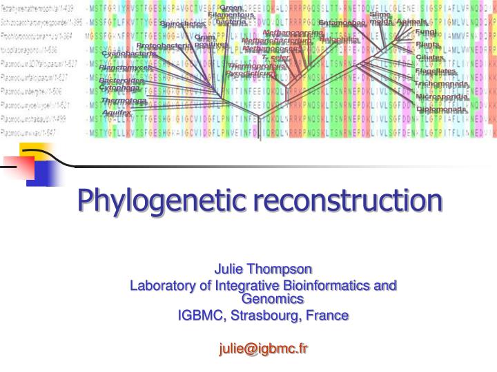
Phylogeneticreconstruction Julie Thompson Laboratory of Integrative Bioinformatics and Genomics IGBMC, Strasbourg, France julie@igbmc.fr
Phylogenetic reconstruction • Introduction: basic concepts • Principal methods for tree reconstruction • Distance based methods • Character based methods • Evaluation of the reliability of a tree • The limits of phylogeny • Some programs
-3 mil yrs AAGACTT AAGACTT -2 mil yrs AAGGCCT AAGGCCT TGGACTT TGGACTT TGGACTT AAGGCCT TGGACTT AAGGCCT -1 mil yrs AGGGCAT AGGGCAT TAGCCCT TAGCCCT AGCACTT AGCACTT AGGGCAT TAGCCCT AGCACTT today AGGGCAT TAGCCCA TAGACTT AGCACAA AGCGCTT Orangutan Gorilla AGGGCAT TAGCCCA TAGACTT AGCACAA AGCGCTT Chimpanzee Human From the Tree of the Life Website, University of Arizona Introduction • What for ? • Reconstruction of evolutionary history of a gene family • Reconstruction of the evolutionary relationships between species : living (extant) and dead (extinct). eg : tree of life • Classification of new species. eg : viral strain • Phylogenetics: the study of evolutionary relatedness among organisms • Relationships represented by a hierarchical, tree-like structure • Originally based on physical similarities and differences (traits or characters) • Now, mostly using gene sequences
Internal node A Leaf node A C B C D root B D Basic concepts : phylogeny • A phylogenetic tree is characterised by : • - its topology (branching patterns) • - the lengths of the branchs (possibly) Rooted tree Unrooted tree Node :represents a taxonomic unit (species, population, gene,…), either existing or ancestor Branch: defines the relationship between the TUs (descent, ancestry) Root : common ancestor of all taxonomic units on tree
A A B B D D E E F F G G A B A B A D B E D D F E E G 0.1 G F 0.1 G F Cladogram Phylogram (branch lengths are not meaningful) (branch lengths are proportional to number of changes) Unrooted tree
Basic concepts : phylogeny For an unrooted tree, there are several possible rooted trees 4 2 C A Position of the root D B 1 5 3 A B C D A B A D C B C C A A C D D B B D 1 2 3 4 5 In most tree reconstruction programs, the position of the root is chosen arbitrarily : - « midpoint rooting » (root placed in the centre of the longest branch) - « outgroup rooting » The user can define the sequence(s) that can be used as an outgroup to root the tree. The outgroup sequence should be distantly related to all other sequences.
Basic concepts : branch order The order of the branchs belonging to the same node is not important. Rotating branchs at a node does not change the topology of the tree. Tree 2 Tree 1 Tree 1 = Tree 2
Homology, orthology, paralogy Homology : 2 genes are homologous if they have a common ancestor Orthology : 2 genes are orthologous if they diverged after a speciation event Paralogy : 2 genes are paralogous if they diverged after a duplication event Ancestral gene of insulin Primates Rodents INS1 INS2 Rat Mouse Rat Mouse INS1 INS2 INS1 INS2 INS Speciation Rat Mouse Rat Mouse Human Duplication
Phylogenetic reconstruction • Introduction: basic concepts • Principal methods for tree reconstruction • Distance based methods • Character based methods • Evaluation of the reliability of a tree • The limits of phylogeny • Some programs
Molecular phylogenetics • DNA, RNA, and protein sequences can be considered as phenotypic traits • Molecular phylogenetics attempts to determine the rates and patterns of change occurring in the sequences and to reconstruct the evolutionary history of genes and organisms • How? • Build a multiple alignment • Validate, edit or mask the resulting alignment • Reconstruct the tree • Evaluate statistically the reliability of the tree
Multiple sequence alignment • Errors in the initial alignment will lead to inaccurate trees Alignment of 18s rRNA sequences (Morrison and Ellis, J Mol Evol, 1997) • alignment algorithms Pileup, ClustalW, TreeAlign, MALIGN, SAM. Trees construction, neighbor-joining, weighted-parsimony, and maximum-likelihood. • different alignments produced trees that were more dissimilar than did the different tree-building methods Using genomic data from seven yeast species (Wong et al, Science 2008) • build alignments using 7 different alignment programs and then estimate phylogeny (using maximum parsimony) • 46.2% of the 1502 genes had one or more differing trees depending on the alignment procedure used Wong, Suchard, Huelsenbeck. Alignment Uncertainty and Genomic Analysis Science, 2008
Alignment masking • Remove or mask columns with gaps and unreliable regions • E.g. Gblocks (Castresana, 2000) Gblocks only Full length alignment
Multiple sequence alignment • The quality of the multiple alignment is crucial for the quality of the tree !! • The trees can vary depending on the region of the alignment selected.
AspRS Anticodon binding domain Catalytic core I Insertion domain Catalytic core II Figure 7 : Représentation schématique des conservations présentes dans les Asp tRNA synthétases après analyse OrdAli. Colonnes noires et grises, résidus strictement conservés ou présents dans au moins 80% des séquences. Colonnes rouges, bleues, jaunes, régions strictement conservées chez les Eucaryotes, Archaea et Bactéries respectivement. Colonnes vertes et violettes, régions communes aux Eucaryotes et Archaea et aux Archaea et bactéries respectivement.
PLASM FALC Whole alignment ARABI THAL Eucarya CAENO ELEG SCHI PO MT DROSO MEGA SACC CE MT MYCOP GENI HOMO SAPIE DROS ME MT RATTU NORV CAEN EL MT MYCOP PNEU Bacteria + Mitochondrie SCHIZ POMB SACCH CERE BORRE BURG CANDI ALBI TREPO PALI MYCOP CAPR BUCHN AFID RICKE PROW RHODO CAPS HALOB SALI CHLOR TEPI ARCHE FULG MYCOB TUBE AQUIF AEOL MYCOB LEPR THERM MARI METBA THER METHA JANN HELIC PYLO PORPH GING CAMPY JEJU Archaea CLOST ACET PYROC KODA CHLAM TRAC BORDE PERT PYROC HORI SYNECHO SP AR THA CHL NEISS GONO NEISS MENI THERM THER DEINO RADI BACIL SUBT PSEUD AERU ENTER FAEC SHEWA PUTR STREP PYOG YERSI PEST ESCHE COLI SALMO TYPH VIBRI CHOL HAEMO INFL ACTIN ACTI
N terminal region Eucarya PLASM FALC SACCH CERE Bacteria Archaea Mitoch. SCHIZ POMB ARABI THAL CANDI ALBI CAENO ELEG DROSO MEGA HALOB SALI HOMO SAPIE PYROC HORI RATTU NORV METBA THER PYROC KODA DROS ME MT METHA JANN SCHI PO MT CAEN EL MT ARCHE FULG BORRE BURG SACC CE MT MYCOP CAPR BUCHN AFID PORPH GING CLOST ACET DEINO RADI RICKE PROW BACIL SUBT RHODO CAPS MYCOP GENI CHLOR TEPI SYNECHO SP MYCOP PNEU CHLAM TRAC BORDE PERT NEISS MENI NEISS GONO HELIC PYLO CAMPY JEJU PSEUD AERU SHEWA PUTR MYCOB TUBE SALMO TYPH ESCHE COLI ENTER FAEC YERSI PEST MYCOB LEPR VIBRI CHOL HAEMO INFL AQUIF AEOL ACTIN ACTI STREP PYOG THERM THER TREPO PALI THERM MARI 0.1 AR THA CHL
Tree reconstruction methods • Distance based methods • UPGMA • Neighbor-Joining • Character based methods • Maximum parsimony • Maximum likelihood
Tree reconstruction methods • Distance based methods • Calculate the distances between pairs of sequences => distance matrix • Group the sequences based on the distances • UPGMA • Neighbor-Joining • relatively simple and fast • but, the sequences themselves are not taken into account
Sites considered : • For DNA, the 3rd base of each codon can be excluded from analysis. • alignment positions with gaps are generally eliminated 2 possibilities : Global gap removal : 18 sites considered Dist(Seq1,Seq2) = 3/18 = 0,1667 Dist(Seq1,Seq3) = 4/18 = 0,2222 Dist(Seq2,Seq3) = 1/18 = 0,0556 Pairwise gap removal : Dist(Seq1,Seq2) = 3/19 = 0,1579 Dist(Seq1,Seq3) = 4/19 = 0,2105 Dist(Seq2,Seq3) = 1/18 = 0,0556 Seq1 MAIKKIISRSNSGIHNATVI Seq2 MPIKK-ISRSNSGIHHSTVI Seq3 MPIKKIISRSNTGI-HSTVI Total sites = 20 No. substitutions (Seq1,seq2) = 3 No. substitutions (Seq1,seq3) = 4 No. substitutions (Seq2,seq3) = 1 Distance calculation Observed distance : mean number of substitutions per site No. substitutions No. sites considered Observed Dist =
Distance correction For more distantly related sequences, the probability of several substitutions occuring at the same site increases. => The number of observed substitutions under-estimates the true number of substitutions between distantly related sequences. Sequence1 Sequence2 Observed no. True no. substitutions substitutions Single substitution C C=>A 1 1 Multiple substitutions C C=>A=>T 1 2 Coincident substitutions C=>G C=>A 1 2 Parallel substitutions C=>A C=>A 0 2 Convergent substitutions C=>A C=>T=>A 0 3 Reverse substitutions C C=>T=>C 0 2 => Numerous methods available that estimate the true distance between sequences
Distance correction: DNA substitution models 3,5 • Jukes-Cantor (JC) model (1969) • The 4 bases have the same frequency • All substitutions occur with equal probabilities • d = -3/4 ln (1-4/3 D) • where D is observed distance 3,0 Jukes-Cantor 2,5 2,0 Corrected distance 1,5 1,0 0,5 0,0 0,00 0,10 0,20 0,30 0,40 0,50 0,60 0,70 Observed distance • Kimura 2 parameter (K2P/K80) model (1980) • The 4 bases have the same frequency • Transitions (sunstitutions A-G or C-T) are more common than transversions • d = - ½ ln(1-2P-Q) – ¼ ln(1-2Q) where P is mean no. of transitions • Q is mean no. of transversions • Tamura-Nei (TrN) model (1993) • 4 bases have different frequencies • different transition frequencies (α1 between purines; α2 between pyrimidines), equal transversion frequencies (β)
Distance calculation: amino acid substitution models • PAM matrices (Dayhoff, 1978) • A 1-PAM mutation matrix describes an amount of evolution which will change, on the average, 1% of the amino acids. In mathematical terms: • estimated from the observation of accepted mutations between 34 superfamilies of closely related sequences • extrapolated to other evolutionary distances (eg. PAM250) • Blosum matrices (1992) • local, ungapped alignments of distantly related sequences to derive the BLOSUM series of matrices. Matrices of this series are identified by a number after the matrix (e.g. BLOSUM50), which refers to the minimum percentage identity of the blocks of multiple aligned amino acids used to construct the matrix. • Gonnet matrices (1992) • similar to Dayhoff, but with more modern sequence databases
UPGMA Method • Group the 2 closest sequences • The node is placed at distance d from each sequence d= (dist seq1,seq2)/2 • Calculate distance between this node and all other sequences : dist (seq1,seq2),seqx = (dist seq1,seqx + dist seq2,seqx) / 2 • etc... UPGMA = Unweighted Pair Group Method with Arithmetic Mean • UPGMA is the simplest clustering algorithm Assumptions : • mutation rate is the same in all ligneages (molecular clock)
1 A 1 B 1 1 A A 1 1 B B 2 2 2 C C D 2 E 1 1 1 1 1 2 2 D D 1 1 2 2 E E 4 F UPGMA Calculation of new distance matrix Distance matrix Clustering A B C D E B 2 C 4 4 D 6 6 6 E 6 6 6 4 F 8 8 8 8 8 dist(A,B),C=(dist AC+dist BC)/2 = 4 dist(A,B),D=(dist AD+dist BD)/2 = 6 dist(A,B),E=(dist AE+dist BE)/2 = 6 dist(A,B),F=(dist AF+dist BF)/2 = 8 dist(D,E),(A,B)=(dist D(A,B)+dist E(A,B))/2 = 6 dist(D,E),C =(dist DC +dist EC )/2 = 6 dist(D,E),F =(dist DF +dist EF )/2 = 8 (A,B) C D E C 4 D 6 6 E 6 6 4 F 8 8 8 8 1 A 1 dist(AB,C),(D,E)=(dist (A,B)(D,E)+dist C(D,E))/2 = 6 dist(AB,C),F =(dist (A,B)F +dist CF )/2 = 8 (A,B) C E C 4 (D,E) 6 6 F 8 8 8 1 B 2 C dist(ABC,DE),F=(dist (AB,C)F+dist(D,E)F)/2=8 (AB,C) (D,E) (D,E) 6 F 8 8 (ABC,DE) F 8
A B C D E B 5 C 4 7 D 7 10 7 E 6 9 6 5 F 8 11 8 9 8 A,C B D E B 6 D 7 10 E 6 9 5 F 8 11 9 8 A,C B D,E B 6 D,E 6.5 9.5 F 8 11 8.5 AC,B D,E D,E 8 F 9.5 9.5 UPGMA Problem : If the mutation rate is different between branches, UPGMA can give a completely false topology Tree obtained by UPGMA Eg: mutation rate of B is much faster than A 2 A 1 2 C 1 3 False topology !! B 0.75 2.5 D 1.5 2.5 E 4.75 F Initial matrix Clustering by UPGMA ACB,DE F 9.5
Neighbor-Joining (NJ) • Reference: Saitou & Nei Mol. Biol. Evol. 4(4):406-25 1987 • Method: • The 2 TUs to be clustered are chosen such that they minimise the sum of lengths of all branchs • The calculation of branch lengths takes into account the mean distance between each sequence and all other sequences => allows different mutation rates between branchs
N S0 = LiX = ( Dij ) / (N-1) i =1 8 i<j 7 1 2 6 X 3 5 4 Neighbor-Joining (NJ) • Estimate sum of branch lengths for all possible clusters (S12,S13,…) => Choose cluster that minimises sum of branch lengths • How to calculate the sum of branch lengths ? For a star-shaped tree, the sum of N branch lengths : Where Dij is distance between TUi and TUj LiX is length between node i and node X
1 2(N-2) N 1 1 S12 = ( D1k+D2k ) +1/2 D12 + Dij N-2 2(N-2) k =3 3 i< j Neighbor-Joining (NJ) Assume TUs 1 and 2 have been joined, then sum of branch lengths : 8 7 1 N 6 S12 = (L1X+L2X) + LXY + LiY X Y i =3 5 2 4 N 3 S12 = D12 + LXY +( Dij) / (N-3) 3 i< j Calcul de LXY : 8 7 N N LXY = [ (D1k+D2k) – (N-2) (L1X+L2X) –2 LiY] In the example : L1Xand L2Xhave been counted 6 times each. Lengths L3Y, …, L8Yhave been counted twice each. Length LXY has been counted 12 times. 1 i =3 k =3 6 X Y 5 2 4 3
Neighbor-Joining (NJ) estimate sum of branch lengths for all possible clusters (S12,S13,…) A B C D E B 5 C 4 7 D 7 10 7 E 6 9 6 5 F 8 11 8 9 8 N 1 1 S12 = ( D1k+D2k ) +1/2 D12 + Dij N-2 2(N-2) k =3 3 i< j Application : SAB = 1/8*62 + 5/2 + 1/4*43 = 21,00 SAC = 1/8*54 + 4/2 + 1/4*52 = 21,75 … Cluster AB
8 1 7 6 X Y 5 2 4 3 Neighbor-Joining (NJ) Branch lengths are estimated by Fitch, Margoliash method (67) L1X = (D12 + D1Z – D2Z) / 2 L2X = (D12 + D2Z – D1Z) / 2 D1Z represents mean distance between 1 and all other sequences D2Z represents mean distance between 1 and all other sequences Application : A B C D E B 5 C 4 7 D 7 10 7 E 6 9 6 5 F 8 11 8 9 8 LAX = (5+6.25-9.25)/2 = 1 LBX = (5+9.25-6.25)/2 = 4 A B => Allows different mutation rates between branchs
Tree reconstruction methods • Distance based methods • UPGMA • Neighbor-Joining => relatively fast and simple => but, the sequences themselves are not taken into account • Character based methods • Each position in the sequence is considered as a trait or character. • maximum parsimony • maximum likelihood • Bayesian inference => calculation time is very long
Maximum Parsimony Used historically to study morphological characters • prefer evolutionary scenario that involves the smallest number of events Application to sequences: • one column in the alignment = one character • Search for most parcimonious trees, i.e. those for which the topology involves minimum number of substitutions Steps : • 1) Search for all possible topologies • 2) either : find smallest no. of substitutions for each topology • or : find informative sites => sites that support one topology
Seq1 Seq3 Seq4 Seq2 Maximum Parsimony First step : find all possible topologies Seq1 AAGAGTGCA Seq2 AGCCGTGCG Seq3 AGATATCCA Seq4 AGAGATCCG AAGAGTGCA 1 AGATATCCA No. of possible topologies (unrooted trees) : 3 AGAGATCCG AGCCGTGCG 3 2 AAGAGTGCA AAGAGTGCA AGCCGTGCG AGCCGTGCG Seq1 Seq1 Seq2 Seq2 Seq4 Seq3 Seq3 Seq4 AGAGATCCG AGATATCCA AGATATCCA AGAGATCCG
Seq1 Seq3 Seq4 {G} G Seq2 {A,G} G {G} G Seq 1 Seq 2 Seq 3 Seq 4 Seq 1 Seq 2 Seq 3 Seq 4 A G G A G G G G 1 substitution Maximum parsimony Second step : find smallest no. of substitutions for a given topology (Fitch method) 1) Root the tree (anywhere) 3) From root to leaves: - Choose one nucleotide x from set N of root n - For child node u, choose one nucleotide : x if x U any nucleotide from set U otherwise AAGAGTGCA AGATATCCA AGA?ATCC? AG??GTGC? AGAGATCCG AGCCGTGCG 2) From leaves to root : Nodes u and v are children of n U,V and N are sets of nucleotides associated with these nodes N= UV if U V ≠ø N= UV otherwise
AAGAGTGCA 1 AGATATCCA Comparison of « length » of tree for the different topologies 4 AGA?ATCC? 2 4 AG??GTGC? AGAGATCCG AGCCGTGCG 10 substitutions 3 2 AAGAGTGCA AAGAGTGCA AGCCGTGCG AGCCGTGCG Seq1 Seq3 Seq1 Seq1 Seq2 Seq2 2 1 5 AGA??T?CA AGA??T?CG 4 5 AGA??T?C? AGA??T?C? 6 Seq4 Seq2 Seq4 Seq3 Seq3 Seq4 AGAGATCCG AGATATCCA AGATATCCA AGAGATCCG 11 substitutions 12 substitutions Maximum parsimony
C D B E A B C B B B A E A A A C C C E E B A D D D E D C B B A A A D C B D D C Search for shortest tree Branch-and-bound Method (Hendy & Penny, 1982) Exact algorithm, guaranteeing the optimal solution without exhaustive searching 1) add sequences one by one (following order of alignment) calculate no. of substitutions for each topology 2) explore different topologies If no. of substitutions during addition > no. found for best topology stop B A C
tree bisection and reconnection subtree pruning and regrafting A3 A2 A5 A5 A2 A4 A1 A4 A1 A6 A6 A3 A3 A3 A4 A5 subtree A7 A7 A2 A2 A4 A5 A1 A1 Search for shortest tree Heuristic methods Can handle more squences and longer sequences, but do not guarantee optimal solution 1) construct initial tree by progressively adding TUs 2) then, rearrange initial tree to reduce length (branch swapping) nearest neighbor interchanges result depends on initial order of sequences perform several tests with different initial ordering : option « jumble »
Seq1 Seq1 Seq1 Seq2 Seq2 Seq3 Seq4 Seq4 Seq3 Seq3 Seq2 Seq4 Seq1 A A GA GT GC A Seq2 A G CC GT GC G Seq3 A G AT AT CC A Seq4 A G AG AT CC G 3 1 1 1 Maximum parsimony Variant : - find all possible topologies - only include informativesites => sites that support one topology 3 2 1
Maximum parsimony Yang J. Mol. Evol.42:294-307 (1996) Gorilla Gorilla Human Human Human Orangutan Chimpanzee Orangutan Gorilla Orangutan Chimpanzee Chimpanzee Topology 3 (13 sites) Topology 2 (9 sites) Topology 1 (17 sites)
Maximum parsimony Problem: long branch attraction C C 3 1 1 3 C C A Parsimonious tree True tree G T 2 4 T G 4 2 G T If the sequences are evolving at very different rates, the probability of convergent substitutions is significant in long branchs => The most parsimonious clustering can lead to false topology • All changes occur at equal rates • no correction for multiple substitutions • Can lead to several equally parsimonious trees • Relatively slow, not suitable for a large number of sequences • No information about branch lengths (generally)
Maximum likelihood • maximizes the probability that a given tree could have produced the observed data (that is, the likelihood) • As for parsimony method : • Each column is considered to be a character • All possible trees are considered • For trees requiring many mutations, probability is low => trees requiring few mutations are preferred • Differences : • Use of an explicit evolutionary model • Allows variablesubstitution rates for each branch • Can be used to estimate reliability of tree
G T T A b c d b a a L5 L6 L4 L3 d c L2 L1 L0 b a c c d a d b Maximum likelihood 3 possible unrooted trees Alignment of 4 sequences 1 2 3 4 Seq a TTGC... Seq b TTGC... Seq c ATAC... Seq d GTAC... tree 3 tree 2 tree 1 tree 1 For position 1, possible combinations of bases at each node : - 3 internal nodes - 4 possible bases at each node No. of possible combinations: 4 x 4 x 4 = 64
G T T A c d b a L5 L6 L4 L3 No of No of possible unrooted trees 3 1 4 3 5 15 6 105 7 945 8 10 395 9 135 135 10 2 027 025 50 >3.1074 G T L2 L1 T L0 Maximum likelihood Estimation of likelihood of tree 1 for position 1 : sum of probabilities for each of 64 combinations Estimation de likelihood of tree 1 : Sum of probabilities obtained for each position Example : The calculation is performed for all possible tree (3 here). The tree with the maximum likelihood is selected. Example of evolutionary model : L0 = frequency of T ~ 0.25 L2 = probability of transversion of T=>G L5 = probability of transition of G=>A L1, L3, L4, L6 = ~1 Probability of this combination for position 1 : L= L0 x L1 x L2 x L3 x L4 x L5 x L6
Bayesian inference • Use Bayes's theorem to combine the prior probability of a phylogeny with the likelihood to produce a posterior probability distribution on trees • Prior probability of a tree before observations are made • (generally, all trees are equally probable) • Likelihood is proportional to probability of the observations, • conditional on the tree (makes assumptions about processes • generating observations) • Posterior probability of a tree is the probability of the tree • conditional on the observations, obtained by combining prior and • likelihood for each tree From Huelsenbeck et al, 2001 Holder & Lewis. Nature Rev. Genet. 2003
Bayesian inference • Choose tree with the highest posterior probability as the best estimate of phylogeny • some numerical methods are available that allow the posterior probability of a tree to be approximated • e.g. Markov chain Monte Carlo (MCMC) in MrBayes (Huelsenbeck et al, 2001)
Phylogenetic reconstruction • Introduction: basic concepts • Principal methods for tree reconstruction • Distance based methods • Character based methods • Evaluation of the reliability of a tree • The limits of phylogeny • Some programs
Evaluation of the reliability of a tree • Goal : Statistically estimate the reliability of a given tree topology • Example : bootstrapping Build n pseudo-alignments by random sampling of the columns in the initial alignment • each column can be used 0,1 or more times • the pseudo-alignments have the same length as the initial alignment • the number of pseudo-alignments should allow for significant statistical testing (n number of columns) • for each pseudo-alignment, build a tree • for each branch in the initial tree, count the number of times this branch is found in the n trees
Evaluation of the reliability of a tree Initial alignment A A B C B 2 C 3 3 D 6 4 4 Seq A A G G C T C C A A A Seq B A G G T T C G A A A Seq C A G C C C C G A A A Seq D A T T T C C G A A C B C D A B A B C B 1 C 6 5 D 8 7 4 Seq A G G G T T T C A A A Seq B G G G T T T G A A A Seq C G C C C C C G A A A Seq D T T T C C C G A A C C 1 D A A 3/3 B B A B C B 2 C 4 2 D 7 5 3 Seq A A T T C C C C A A A Seq B A T T C C G G A A A Seq C A C C C C G G A A A Seq D A C C C C G G C C C C C 2 D D A A B C B 1 C 3 2 D 6 5 3 Seq A A G T T C C C A A A Seq B A G T T C C G A A A Seq C A G C C C C G A A A Seq D A T C C C C G A C C B C 3 D Random sampling
Archaea 26 Eucarya 100 Archaea 34 bootstrap value of a node is the percentage of times that node is present in the trees built from the random samples 100 Phylogenetic tree of the ribosomal proteins L2p Bacteria
Phylogenetic reconstruction • Introduction: basic concepts • Principal methods for tree reconstruction • Distance based methods • Character based methods • Evaluation of the reliability of a tree • The limits of phylogeny • Some programs