Download
1 / 47
500 likes | 701 Views
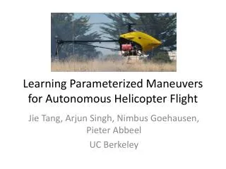
Machine Learning Techniques For Autonomous Aerobatic Helicopter Flight. Joseph Tighe. Helicopter Setup. XCell Tempest helicopter Micorstrain 3DM-GX1 orientation sensor Triaxial accelerometers SP? Rate gyros Magnetometer Novatel RT2 GPS.

E N D
Machine Learning Techniques For Autonomous Aerobatic Helicopter Flight Joseph Tighe
Helicopter Setup • XCell Tempest helicopter • Micorstrain 3DM-GX1 orientation sensor • Triaxial accelerometers SP? • Rate gyros • Magnetometer • Novatel RT2 GPS
What are some differences between this problem and ones we’ve seen so far? Static Learning Learning Control • Set training and testing set • Try to “learn” from the training set to predict the testing set • The task we are learning is static (does not change from one trial to the next) • Training set can still be known upfront • No testing set • We are learning how to perform a dynamic task, we need to be able to adapt to changes mid task
Helicopter Environment and Controls • To fully describe the helicopter’s “state” mid-flight: • Position: (x, y, z) • Orientation (expressed as a unit quaternion) • Velocity (x’, y’, z’) • Angular velocity(x y z) • The helicopter can be controlled by: • (u1, u2): Pitch • (u3): Tail Rotor • (u4): Collective pitch angle
What is needed to fly autonomous? • Trajectory • The desired path for the helicopter to follow • Dynamics Model • Inputs: current state and controls (u1, u2, u3, u4) • Output: predicts where the helicopter will be at the next time step • Controller • The application the feeds the helicopter the correct controls to fly the desired trajectory
Trajectory • A path through space that fully describes the helicopter's flight. • It is specified by a sequence of states that contain: • Position: (x, y, z) • Orientation (expressed as a unit quaternion) • Velocity (x’, y’, z’) • Angular velocity(x y z) • For flips this is relatively simple to encode by hand • Later we will look at a way to learn this trajectory from multiple demonstrations of the same maneuver
Simple Dynamics Model (Car) • What state information is needed?: • Position on ground (x, y) • Orientation on ground () • Speed (x’, y’) • What are the controls? • Current gear • Accelerator/Break • Steering wheel position • What would the dynamics model do? • Given state and control compute an acceleration vector and angular acceleration vector
Helicopter Dynamics Model • Our state and controls are more complicated than the car example. • There are also many hidden variables that we can’t expect to model accurately. • Air, rotor speed, actuator delays, etc. • Conclusion: much harder problem than the car example • we’ll have to learn the model
Controller • Given a target trajectory and current state compute the best controls for the helicopter. • Controls are (u1, u2, u3, u4) • (u1, u2): Pitch • (u3): Tail Rotor • (u4): Collective pitch angle
Overview of the two approaches • Given one example flight and target trajectory specified by hand, learn a model and controller that can fly the trajectory • Given a number of example flights of the same maneuver, learn the trajectory, model and controller that can fly the trajectory.
Approach 1: Known Trajectory P. Abbeel, A. Coates, M. Quigley, and A. Ng, An Application of Reinforcement Learning to Aerobatic Helicopter Flight, NIPS 2007
Overview Dynamics Model Data Known Trajectory + Penalty Function Reward Function Reinforcement Learning Policy We want a robot to follow a desired trajectory. Slide taken from: A. Coates, P. Abbeel, and A. Ng, Learning for Control from Multiple Demonstrations, ICML 2008
Markov Decision Processes • Modeled as a sextuple (S, A, P(·|·, ·), H, s(0), R) • S: All possible states of our system • A: All possible actions we can perform • P(s’| s, a): The probability that an action a in state s at a time t will lead to s’ at time t+1. • H: The time over which the system will run (not strictly needed) • s(0): The start state • R(a, s, s’): is the reward for transitioning from state s to s’ after taking action a. This function can be unique for each time step t.
Markov Decision Processes • Once we have this model we wish to find a policy, (s), that maximizes the expected reward • (s) is a mapping from the set of states S to the set of action A, with a unique mapping for each time step. • V(s’) is sum of rewards achieved by following from s’
Back to helicopter modeling • For our problem: • S: is the range of orientations and speeds that are allowed • A: is our range of control inputs • H: The length of our trajectory • s(0): Where the helicopter starts • P(s’|s, a): Our dynamics model (unknown) • R(a, s, s’): Tied to the desired trajectory (trivially computed) • (s): Our controller (unknown)
Overview Dynamics Model Data Known Trajectory + Penalty Function Reward Function Reinforcement Learning Policy We want a robot to follow a desired trajectory. Slide taken from: A. Coates, P. Abbeel, and A. Ng, Learning for Control from Multiple Demonstrations, ICML 2008
Reinforcement Learning • Tries to find a policy that maximizes the long term reward of an environment often modeled by a MDP. • First an exploration phase explores state/action pairs whose transition probabilities are still unknown. • Once the MDP transition probabilities are modeled well enough an exploitation phase maximizes the sum of rewards over time.
Exploration vs Exploitation • More exploration will give a more accurate MDP model • More exploitation will give a better policy for the given model • What issues might we have with exploration stage for our problem? • Aggressive exploration can cause the helicopter to crash
Apprenticeship Learning • Exploration: Start with an example flight • Compute a dynamics model and reward function based on the target trajectory and sample flight • Giving you a MDP model • Exploitation:Find a controller (policy: ) that maximizes this reward • Exploration:Fly the helicopter with the current controller and add this data to the sample flight data • If we flew the target trajectory stop, otherwise go back to step 2
Dynamics Model • Linear model • We must learn parameters: A, B, C, D, E • g: gravity field • b: body coordinate frame • w: Gaussian random variable Forward Sideways Up/Down Figure taken from: P. Abbeel, A. Coates, M. Quigley, and A. Ng, An Application of Reinforcement Learning to Aerobatic Helicopter Flight, NIPS 2007
Approach 2: Learn Trajectory A. Coates, P. Abbeel, and A. Ng, Learning for Control from Multiple Demonstrations, ICML 2008.
Learning Trajectory and Controller Dynamics Model Data Trajectory + Penalty Function Reward Function Reinforcement Learning Policy We want a robot to follow a desired trajectory. Slide taken from: A. Coates, P. Abbeel, and A. Ng, Learning for Control from Multiple Demonstrations, ICML 2008
Key difficulties • Often very difficult to specify trajectory by hand. • Difficult to articulate exactly how a task is performed. • The trajectory should obey the system dynamics. • Use an expert demonstration as trajectory. • But, getting perfect demonstrations is hard. • Use multiple suboptimal demonstrations. Slide taken from: A. Coates, P. Abbeel, and A. Ng, Learning for Control from Multiple Demonstrations, ICML 2008
Problem Setup • Given: • Multiple demonstrations of the same maneuver • s: sequence of states • u: control inputs • M: number of demos • Nk: length of demo k for k =0..M-1 • Goal: • Find a “hidden” target trajectory of length T
Graphical model Intended trajectory • Intended trajectory satisfies dynamics. • Expert trajectory is a noisy observation of one of the hidden states. • But we don’t know exactly which one. Expert demonstrations Time indices Slide taken from: A. Coates, P. Abbeel, and A. Ng, Learning for Control from Multiple Demonstrations, ICML 2008
Learning algorithm • Make an initial guess for . • Alternate between: • Fix . Run EM on resulting HMM. • Choose new using dynamic programming. If is unknown, inference is hard. If is known, we have a standard HMM. Slide taken from: A. Coates, P. Abbeel, and A. Ng, Learning for Control from Multiple Demonstrations, ICML 2008
Algorithm Overview • Make initial guess for : say a even step size of T/N • E-Step: Find a trajectory by smoothing the expert demonstrations • M-step: With this trajectory update the covariances using the standard EM update • E-Step: run dynamic time warping to find a that maximizes the P(z, y) or the probability of the current trajectory and expert examples • M-Step: Find d given . • Repeat steps 2-5 until convergence
Dynamic Time Warping • Used in speech recognition and biological sequence alignment (Needleman-Wunsch) • Given a distribution of time warps (d) dynamic programming is used to solve for . Figure taken from: A. Coates, P. Abbeel, and A. Ng, Learning for Control from Multiple Demonstrations, ICML 2008
Results for Loops Figure taken from: A. Coates, P. Abbeel, and A. Ng, Learning for Control from Multiple Demonstrations, ICML 2008
Details: Drift • The various expert demonstrations tend to drift in different ways and at different time. • Because these drift errors are highly correlated between time steps Gaussian noise does a poor job of modeling them • Instead drift is explicitly modeled by slow changing translation in space for each time point.
Details: Prior Knowledge • It is also possible to incorporate expert advice or prior knowledge • For example: flips should keep the helicopter center fixed in space or loops should lie on a plane in space • This prior knowledge is used as additional constrains in both EM steps of the algorithm
Dynamics Model Dynamics Model Data Trajectory + Penalty Function Reward Function Reinforcement Learning Policy Slide taken from: A. Coates, P. Abbeel, and A. Ng, Learning for Control from Multiple Demonstrations, ICML 2008
Standard modeling approach • Collect data • Pilot attempts to cover all flight regimes. • Build global model of dynamics 3G error! Slide taken from: A. Coates, P. Abbeel, and A. Ng, Learning for Control from Multiple Demonstrations, ICML 2008
Errors aligned over time • Errors observed in the “crude” model are clearly consistent after aligning demonstrations. Slide taken from: A. Coates, P. Abbeel, and A. Ng, Learning for Control from Multiple Demonstrations, ICML 2008
New Modeling Approach • The key observation is that the errors in the various demonstrations are the same. • This can be thought of as reveling the hidden variables discussed earlier: • Air, rotor speed, actuator delays, etc. • We can use this error to correct a “crude” model.
Time-varying Model • f: is the “crude” model • : is the bias computed by the difference between the crude model predicted trajectory and the target trajectory in a small window of time around t. • : Gaussian noise
Final Dynamics Model Data Trajectory + Penalty Function Reward Function Reinforcement Learning Policy Slide taken from: A. Coates, P. Abbeel, and A. Ng, Learning for Control from Multiple Demonstrations, ICML 2008
Summary • The trajectory, dynamics model and controller are all learned • The dynamics model is specific to a portion of the maneuver being performed
Compare Two Techniques Technique 1 Technique 2 • Hand specified trajectory • Learn global model and controller • For a new maneuver: an example flight must be given and new trajectory specified • Learn trajectory, time varying model and controller • For a new maneuver: a couple of example flights must be given + 30 min of learning