Download

1 / 44
490 likes | 690 Views
Introduction to Model Initialization. 26 November 2012. Thematic Outline of Basic Concepts. What is meant by numerical model initialization? What data are available to initialize a numerical model simulation, and what are the caveats that influence their use for model initialization?

E N D
Introduction to Model Initialization 26 November 2012
Thematic Outline of Basic Concepts • What is meant by numerical model initialization? • What data are available to initialize a numerical model simulation, and what are the caveats that influence their use for model initialization? • What is model spin-up and its impacts upon NWP? • What are some commonly-used methods for observational targeting to improve forecast skill?
Initialization: the process by which observations are processed to define the initial conditions for a model’s dependent variables (where processed infers taking observations, performing quality control, assimilating the observations, and ensuring that the final analysis is balanced and representative of the real atmosphere)
Types of Model Initialization • Static Initialization: interpolation (or downscaling) of data to a model grid and subsequent adjustment as necessary to meet a desired balance condition. • Example: using another model’s initial analysis as initial conditions for a limited area model simulation. • Dynamic Initialization: use of a numerical model during a preforecast period to assimilate data, ensure balance, and to spin-up small-scale features. • We’ll focus on this method through the rest of this chapter.
Types of Observations • In Situ: locally-measured observations • Remotely Sensed: observations measured from afar • Active remote sensing: a sensor emits radiation energy and measures the atmospheric response to that radiation • Passive remote sensing: a sensor only measures naturally-emitted radiation; it emits no radiation of its own • Examples of both types of observations may be found in Section 6.2.1 of the course text.
Remotely Sensed Data • A remote sensing platform measures radiation energy and how it is impacted by atmospheric phenomena. • Attenuation, phase delay, etc. • It does not directly observe dependent model variables. • What the remote sensing platform measures can be related to the dependent model variables through the use of a physically-based retrieval algorithm.
Remotely Sensed Data • With non-variational data assimilation, a retrieval algorithm is used to obtain values for dependent meteorological variables prior to assimilation. • With variational data assimilation, the retrieval algorithm is encompassed within the assimilation code, allowing the direct use of remotely sensed data.
Remotely Sensed Data Concern #1: Observation Uncertainty • All measurements are associated with observational error inherent to the observing platform. • In addition, retrieval algorithms inherently introduce observation uncertainty due to sensitivities in their formulations to specific atmospheric constituents. • Example: GPS radio occultations and moisture content
Remotely Sensed Data Concern #2: Vertical Extent of Data • Satellite-based remote sensing platforms are great for measuring upper atmospheric conditions. • However, they are often strongly impacted by clouds and precipitation. This can limit their ability to gather observations in the lower to middle troposphere.
Remotely Sensed Data Benefit: Spatial and Temporal Resolution • Radar and geostationary remote sensing platforms have relatively high spatial and temporal resolution. • Space: roughly 250 m-4 km (horizontal), < 1 km (vertical) • Time: roughly 1-30 minutes • Polar-orbiting sensors have similar resolution but cover a changing area of limited extent in each scan.
In Situ Data Concern #1: Data Representativeness • Since the observation is a point observation, it may be of local variability that is not representative of the atmosphere as resolved by the numerical model. • Upper tropospheric example: mountain wave • Lower tropospheric example: boundary layer eddies • Surface observations thus pose a particular assimilation challenge. • When temporal availability permits, temporally-averaging over some representative interval may help mitigate this problem.
In Situ Data Concern #2: Data Density • Observation platforms are often tightly clustered around where people are located. • Thus, relatively few observations are available over sparsely-populated land areas and over water.
In Situ Data Concern #3: Temporal Availability • For selected platforms, data are not always available. • Radiosondes: data typically available only every 12 h • Aircraft: limited over infrequently-flown flight routes • Numerous other issues can impact data availability, particularly from lesser-developed regions. • Staffing of observing station (day vs. night, political unrest) • Instrument malfunctions, data communication delays
In Situ Data Concern #4: Data Quality • Observation error is endemic to all instruments, the magnitude of which varies from station to station. • Poorly-sited instruments can bias the data to being unrepresentative of the region. • Example: bank thermometers (notoriously bad!)
Quality Control • Quality Control: the protocols used to ensure that a given observation is of sufficiently high quality to be used within a numerical model analysis. • There are many possible means by which an individual observation may be erroneous. • Independent of inherent observational error/uncertainty. • Specific examples are contained on the next slide.
Quality Control • Improper Data Transmission • Time, date, and/or location information may be incorrect. • Data may become corrupted upon transmission. • Systematic Errors (improper instrument calibration) • Random Errors (instrument malfunction) • Representativeness Errors (discussed earlier)
Quality Control Methods • Limit Tests • Sensor Limits: Is the reported value outside of the range of values that the instrument can accurately measure? • Climatological Limits: Is the reported value well outside of the range of previously-observed values at that station? • Must be careful with such a test, however, for rare events! • Physical Limits: Is the reported value outside of the range of physically-realistic values? (e.g., negative wind or RH)
Quality Control Methods • Temporal Consistency Checks • Is the reported value smoothly-varying or rapidly fluctuating in time for reasons independent of the underlying meteorological conditions? • Spatial Consistency Checks • Is the reported value in reasonable agreement (independent of local variability) with either nearby observations or the first guess atmospheric state estimate?
Quality Control • A quality control protocol must have the following three characteristics… • Flexible: It must be able to handle multiple observation types from multiple sensors in multiple locations. • Accurate: It must be able to discard erroneous data while keeping good data, even if it is unusual for a given location. • Automateable: It must be largely automated given the large amounts of data that are routinely available.
Quality Control • The erroneous discarding of a good observation can have as much of a negative impact upon an initial atmospheric analysis as keeping a bad observation! • Example: January 24-25, 2000 East Coast Blizzard • Notable 6-18 h regional and global NWP failure • Most quality control systems discarded the Little Rock, AR sounding, which sampled an intense, local jet streak. • In actuality, the observation was accurate and should not have been discarded!
Quality Control (Image obtained from Storm Prediction Center)
Quality Control 300 hPa Wind Differences (With LZK Observation Minus Without LZK Observation) Top: Compared to Operational Eta Analysis > 12 m s-1! Bottom: Compared to Operational ECMWF Analysis > 15 m s-1! (Zhang et al. 2002, Mon. Wea. Rev., Figure 10)
Model Spin-Up • Atmospheric variability typically occurs on scales smaller than those that our observing network can reasonably resolve. • A numerical model may be able to resolve such variability, whether crudely or otherwise. • However, if a static initialization is employed, such variability will be absent from the initial conditions.
Model Spin-Up • Once the model begins its forecast period, it will generate such atmospheric variability. • However, it takes time for the variability to mature (e.g., become physically-realistic and balanced). • The process by which such variability is generated is known as model spin-up. The time taken to generate such variability is the model spin-up period (~6-12 h).
Model Spin-Up • Forecast data from the spin-up period is typically discarded. Thus, a static initialized simulation should start >12 h prior to the forecast period of interest. • Dynamical initializations utilize a pre-forecast integration period coupled with data assimilation at the end of that period. • Pre-forecast integration: spin-up the model • Data assimilation: correct or adjust the estimate of the atmospheric state at the ‘initial’ forecast time (t = 0)
Model Spin-Up Terminology • Cold Start: analogous to a static initialization • Warm Start: a partially spun-up initial condition from a dynamic initialization • In current-generation NWP models, typically includes only kinematic features and not precipitation active at t = 0. • Hot Start: a fully spun-up initial condition from a dynamic initialization • Includes both kinematic and precipitating features.
Targeted Observations • Typically, forecasts benefit from increased observation density. • For numerous reasons, this is typically only realistic ahead of high-impact events or during field programs. • Observation targeting describes the processes by which the siting of additional observations may be determined to provide optimal forecast benefit.
Targeted Observations Example: Hurricane Sandy, 1200 UTC 23 October 2012 GFS Ensemble Forecast
Targeted Observations • Track forecasts are tightly clustered through 120 h. • Let’s say that we want to reduce forecast spread and increase forecast skill at 144 h (1200 UTC 29 October 2012, about 12 h prior to landfall). • Our observation targeting method must highlight where observations should be collected in the short-term to most positively impact the next forecast cycle’s track forecast for 1200 UTC 29 October 2012.
Targeted Observations improved forecast quality via observation targeting (decreased RMS forecast error with obs) degraded forecast quality via observation targeting (increased RMS forecast error with obs)
Targeted Observations • Method 1: Ensemble Variance/Spread • Gather additional observations where the greatest short-range ensemble forecast spread is realized. • Assumptions… • Error growth is greatest where the initial condition uncertainty is highest. • The uncertainty propagates forward in time (and space) within successive analysis cycles until ‘corrected’ by obs.
Targeted Observations • Method 2: Adjoint Methods • Relates an analysis metric over the model domain to a desired forecast field over a specific region. • Utilizes a numerical model forecast to compute the sensitivity of the forecast field to small, arbitrary perturbations in the analysis metric. • If forecast spread due to small perturbations in the initial conditions is large, we want to make the initial conditions more certain in order to constrain/improve the forecast!
Adjoint Methods Step 4: Conduct Non-Linear Model Forecast Step 3: Acquire Observations Step 2: Integrate Adjoint Model Step 1: Integrate Forward Linear (Often Dry) Model ti = 0 ta = 36 h tv = 84 h ti = initial time, ta = adjoint/analysis time, tv = verifying time
Adjoint Methods Sensitivity of 72-h ζ in • area in (a) Left: Sensitivity to perturbed 400 hPa v (ICs) at 0 h Right: Sensitivity to perturbed 400 hPa v (LBCs) at 0 h Note difference in contour intervals between panels!
Adjoint Methods • In this case, the greatest impact upon the 72-h ζ forecast would be manifest by gathering observations along the lateral boundaries (e.g., west of CA). • Note that this is specific to the model being used here; the same may not hold true for other models, model configurations, or the real atmosphere!
Adjoint Methods • Such observations could then be assimilated at a later time (e.g., t = 24 h), to launch a 48-h forecast. • Note: Table 3.2 – sensitivity in the area of the lateral boundary conditions is even higher at t = 24 h than at t = 0. • The theoretical improvement in the quality of the initial conditions should, theoretically, improve the quality of the ζ forecast valid at t = 72 h.
Targeted Observations • Method 3: Ensemble Kalman Filter & Related Tools • Rather than assess the sensitivity to small, arbitrary initial condition perturbations to a deterministic analysis, do so in the context of an ensemble. • Initial condition spread is manifest through the ensemble, which is derived from a cycled data assimilation system. • Uncertainty is thus a function of the available observations and the forward propagation of initial condition errors.
Ensemble Targeting Methods Here, we focus on the Ancell and Hakim (2007, MWR) method for defining the ensemble sensitivity metric: J = forecast metric with the ensemble mean removed J = ensemble mean value of J x = analysis state variable with the ensemble mean removed x = ensemble mean value of x cov() = covariance, var() = variance
Ensemble Targeting Methods • This provides a quantification of the sensitivity of J to uncertainty in the initial condition given by x. • Nominally, J is taken to be some field of interest over some specific region of interest. • Conversely, x is taken over the entirety of the domain, one variable at a time. There may be many different x for a given J!
Ensemble Targeting Methods • Uniquely, these methods allow for the estimation of how a hypothetical observation (in x) will impact the forecast value of J. • In other words, this provides a priori information about how a targeted observation would impact the forecast! • As with adjoint methods, the idea is to make the initial conditions more certain to better hone in on the ‘correct’ forecast, though this method too is model-dependent. • More details: see works by Ryan Torn or Fuqing Zhang
Targeted Observations • Method 4: Subjective Methods • Presumably, forecast sensitivity is greatest to uncertainty in the initial conditions manifest where atmospheric gradients are the sharpest. • Identification of such areas from available observations or syntheses thereof can be used to subjectively identify observation gathering locations. • May or may not improve a given model’s forecast, however!