Download
1 / 20
400 likes | 820 Views
A finite element approach for modeling Diffusion equation. Subha Srinivasan 10/30/09. Forward Problem Definition.

E N D
A finite element approach for modeling Diffusion equation SubhaSrinivasan 10/30/09
Forward Problem Definition • Given a distribution of light sources on the boundary of an object and a distribution of tissue parameters within , to find the resulting measurement set on
Inverse Problem Definition • Given a distribution of light sources and a distribution of measurements on the boundary , to derive the distribution of tissue parameters within
Diffusion equation in frequency domain • is the isotropic fluence, is the Diffusion coefficient, is the absorption coefficient and is the isotropic source • is the reduced scattering coefficient
Solutions to Diffusion equation • Analytical solutions exist in simple geometries • Finite difference methods (FDM) use approximations for differentiation and integration. Works well for 2D problems with regular boundaries parallel to coordinate axis, cumbersome for regions with curved or irregular boundaries • Finite element methods (FEM) can be easily applied to complicated and inhomogeneous domains and boundaries. Versatile and computationally feasible (compared to Monte Carlo methods)
Using FEM for Modeling • Main concept: divide a volume/area into elements and build behavior in entire area by characterizing each element (Mosaic) • Uses integral formulation to generate a set of equations • Uses continuous piecewise smooth functions for approximating unknown quantities
Basis Functions For a set of basis functions, we can choose anything. For simplicity here, shown are piecewise linear “hat functions”. Our solution will be a linear combination of these functions. φ3 φ1 φ2 x1=0 x2=L/2 x3=L
Derivation of FEM formulation for Diffusion Equation • The approximate solution is: • And for flux: • Galerkin formulation gives the weighted residual to equal zero: • Galerkin weak form: • Green’s identity: • Substituting:
Matrix form of FEM Model • Discretizing parameters: • Overall: • Matrix form: • For A,B detailed, refer to Paulsen et al, Med Phys, 1995 • Need to apply BCs
Boundary Conditions • Type III BC, Robin type • α incorporates reflection at the boundary due to refractive index change
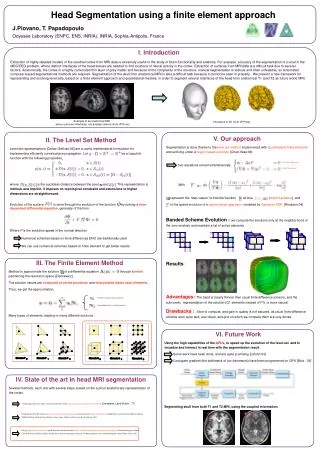
Source Modeling • Point source: contribution of source to element in which it falls • Gaussian source: modeled with known FWHM • Distributed source model: • Hybrid monte-carlo model: Monte carlo model close to source & diffusion model away from source Paulsen et al, Med Phys, 1995
Hybrid Source Model Ashley Laughney summer project, 2007
Plots near the source Ashley Laughney summer project, 2007
References • Arridge et al, Med Phys, 20(2), 1993 • Schweiger et al, Med Phys, 22(11), 1995 • Paulsen et al, Med Phys, 22(6), 1995 • Wang et al, JOSA(A), 10(8), 1993