Download
1 / 13
130 likes | 245 Views
0. 0. 1. 3. 1. 3. 2. 2. Directed graph (digraph): < v i , v j > ::= < v j , v i >. tail. head. v i. v j. 0. 0. 1. 1. 2. CHAPTER 9 GRAPH ALGORITHMS. §1 Definitions.

E N D
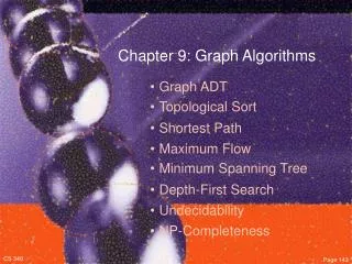
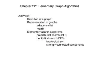
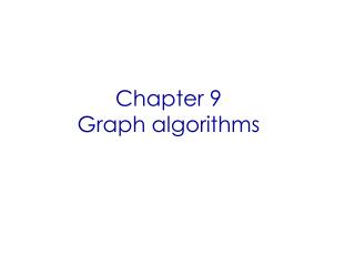
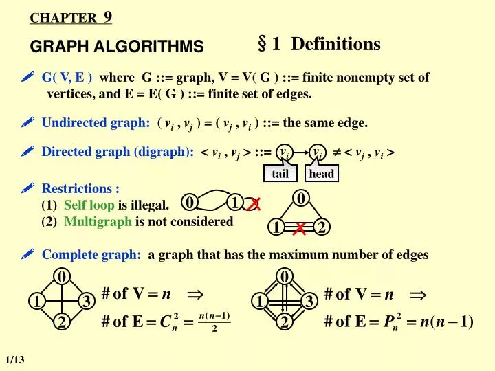
0 0 1 3 1 3 2 2 Directed graph (digraph): <vi , vj > ::= < vj , vi > tail head vi vj 0 0 1 1 2 CHAPTER 9 GRAPH ALGORITHMS §1 Definitions G( V, E ) where G ::= graph, V = V( G ) ::= finite nonempty set of vertices, and E = E( G ) ::= finite set of edges. Undirected graph: ( vi , vj ) = ( vj , vi ) ::= the same edge. Restrictions : (1) Self loop is illegal. (2) Multigraph is not considered Complete graph: a graph that has the maximum number of edges 1/13
§1 Definitions vi and vj are adjacent ; ( vi , vj ) is incident onvi and vj vi vj vi is adjacenttovj; vj is adjacentfromvi; < vi , vj > is incident onvi and vj vi vj Subgraph G’ G ::= V( G’ ) V( G ) && E( G’ ) E( G ) Path ( G) from vpto vq::= { vp, vi1, vi2, , vin, vq } such that ( vp, vi1 ), ( vi1, vi2 ), , ( vin, vq ) or < vp, vi1 >, , < vin, vq > belong to E( G ) Length of a path ::= number of edges on the path Simple path::= vi1, vi2, , vin are distinct Cycle::= simple path with vp= vq viand vjin an undirected G areconnectedif there is a path from vito vj(and hence there is also a path from vjto vi) An undirected graph G isconnectedif every pair of distinct viand vjare connected 2/13
§1 Definitions v Given G with n vertices and e edges, then (Connected) Component of an undirected G::= the maximal connected subgraph A tree ::= a graph that is connected and acyclic A DAG ::= a directed acyclic graph Strongly connected directed graph G ::= for every pair of viand vjin V( G ), there exist directed paths from vito vjand from vjto vi. If the graph is connected without direction to the edges, then it is said to be weakly connected Strongly connected component ::= the maximal subgraph that is strongly connected Degree( v )::= number of edges incident to v. For a directed G, we have in-degree and out-degree. For example: in-degree(v) = 3; out-degree(v) = 1; degree(v) = 4 3/13
§1 Definitions Representation of Graphs Adjacency Matrix adj_mat [ n ] [ n ] is defined for G(V, E) with n vertices, n 1 : Hey you begin to know me! Right. And it wastes time as well. If we are to find out whether or not G is connected, we’ll have to examine all edges. In this case T and S are both O( n2 ) I know what you’re about to say: this representation wastes space if the graph has a lot of vertices but very few edges, right? The trick is to store the matrix as a 1-D array: adj_mat [ n(n+1)/2 ] = { a11, a21, a22, ..., an1, ..., ann } The index for aijis ( i ( i 1 ) / 2 + j ). Note: If G is undirected, then adj_mat[ ][ ] is symmetric. Thus we can save space by storing only half of the matrix. 4/13
§1 Definitions 0 1 2 graph[2] graph[1] graph[0] 0 2 1 Adjacency Lists Replace each row by a linked list 〖Example〗 Note: The order of nodes in each list does not matter. For undirected G: S = nheads + 2enodes = (n+2e) ptrs+2e ints 5/13
§1 Definitions 0 1 2 inv[2] inv[0] inv[1] 1 1 0 tail i head j row for tail column for head Degree( i ) = number of nodes in graph[ i ] (if G is undirected). Tof examine E(G) = O( n + e ) If G is directed, we need to find in-degree(v) as well. Method 1 Add inverse adjacency lists. 〖Example〗 Method 2 Multilist (Ch 3.2) representation for adj_mat[ i ] [ j ] 6/13
§1 Definitions graph[j] graph[i] graph[j] graph[i] …… …… i j mark v1 v2 graph[0] 0 graph[1] node next v1 next v2 1 2 graph[2] 3 0 2 0 1 2 3 graph[3] Adjacency Multilists In adjacency list, for each ( i, j ) we have two nodes: Now let’s combine the two nodes into one: Wait a minute ... Look at the space taken: (n+2e) ptrs + 2e ints and “mark” is not counted. What’s the advantage? 〖Example〗 Sometimes we need to mark the edge after examine it, and then find the next edge. This representation makes it easy to do so. Weighted Edges adj_mat [ i ] [ j ] = weight adjacency lists \ multilists : add a weight field to the node. 7/13
§2 Topological Sort 〖Example〗 Courses needed for a computer science degree at a hypothetical university How shall we convert this list into a graph? 8/13
§2 Topological Sort AOV Network ::= digraph G in which V( G ) represents activities ( e.g. the courses ) and E( G ) represents precedence relations ( e.g. means that C1 is a prerequisite course of C3 ). C1 C3 i is a predecessor of j ::= there is a path from i to j i is an immediate predecessor of j ::= < i, j > E( G ) Then j is called a successor ( immediate successor ) of i Partial order ::= a precedence relation which is both transitive ( i k, k j i j ) and irreflexive ( i i is impossible ). Note: If the precedence relation is reflexive, then there must be an i such that i is a predecessor of i. That is, i must be done before i is started. Therefore if a project is feasible, it must be irreflexive. Feasible AOV network must be a dag (directed acyclic graph). 9/13
§2 Topological Sort 【Definition】A topological order is a linear ordering of the vertices of a graph such that, for any two vertices, i, j, if i is a predecessor of j in the network then i precedes j in the linear ordering. 〖Example〗One possible suggestion on course schedule for a computer science degree could be: 10/13
§2 Topological Sort Note: The topological orders may not be unique for a network. For example, there are several ways (topological orders) to meet the degree requirements in computer science. Test an AOV for feasibility, and generate a topological order if possible. Goal void Topsort( Graph G ) { int Counter; Vertex V, W; for ( Counter = 0; Counter < NumVertex; Counter ++ ) { V = FindNewVertexOfDegreeZero( ); if ( V == NotAVertex ) { Error ( “Graph has a cycle” ); break; } TopNum[ V ] = Counter; /* or output V */ for ( each W adjacent to V ) Indegree[ W ] – – ; } } /* O( |V| ) */ T = O( |V|2 ) 11/13
§2 Topological Sort v1 v2 v3 v4 v5 Indegree v1 0 v2 1 v6 v7 v3 2 v4 3 v5 1 v6 3 v7 2 Improvement: Keep all the unassigned vertices of degree 0 in a special box (queue or stack). Mistakes in Fig 9.4 on p.289 void Topsort( Graph G ) { Queue Q; int Counter = 0; Vertex V, W; Q = CreateQueue( NumVertex ); MakeEmpty( Q ); for ( each vertex V ) if ( Indegree[ V ] == 0 ) Enqueue( V, Q ); while ( !IsEmpty( Q ) ) { V = Dequeue( Q ); TopNum[ V ] = ++ Counter; /* assign next */ for ( each W adjacent to V ) if ( – – Indegree[ W ] == 0 ) Enqueue( W, Q ); } /* end-while */ if ( Counter != NumVertex ) Error( “Graph has a cycle” ); DisposeQueue( Q ); /* free memory */ } T = O( |V| + |E| ) Home work: p.339 9.2 What if a stack is used instead of a queue? v6 v7 0 v3 1 0 v4 2 0 1 v5 0 2 1 0 v2 1 0 v1 12/13
Laboratory Project 3 Hashing Due: Wednesday, November 4th, 2009 at 10:00pm Detailed requirements can be downloaded from http://acm.zju.edu.cn/dsaa/ Don’t forget to sign you names and duties at the end of your report. 13/13