Critical Region

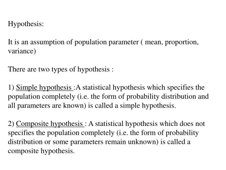
1. Hypothesis:It is an assumption of population parameter ( mean, proportion, variance)There are two types of hypothesis :1) Simple hypothesis :A statistical hypothesis which specifies the population completely (i.e. the form of probability distribution and all parameters are known) is called a simple hypothesis.2) Composite hypothesis : A statistical hypothesis which does not specifies the population completely (i.e. the form of probability distribution or some parameters remain unknown) is called a composite hypothesis.

2. Hypothesis Testing or Test of Hypothesis or Test of Significance : Hypothesis testing is a process of making a decision on whether to accept or reject an assumption about the population parameter on the basis of sample information at a given level of significance.Null Hypothesis : It is the assumption which we wish to test and whose validity is tested for possible rejection on the basis of sample information.It is denoted by HoAlternative Hypothesis : It is the hypothesis which differs from the null hypothesis. It is not tested It is denoted by H1 orHaLevel of significance : It is the maximum probability of making a type I error when the null hypothesis is true as an equality.

3. It is usually expressed as % and is denoted by symbol α( called alpha)It is used as a guide in decision making. It is used to indicate the upper limit of the size of the critical regionTEST STATISTIC

4. Critical Region or Rejection Region :Critical region is the region which corresponds to a pre-determined level of significance. The set of value of the test statistic which leads to rejection of the null hypothesis is called region of rejection or Critical region of the test. Conversely the set of values of the test statistic which leads to the acceptance of Ho is called region of acceptance.Critical Value :It is that value of statistics which separate the critical region from the acceptance region. It lies at the boundary of the regions of acceptance and rejection.Size of critical region :The probability of rejecting a true null hypothesis is called as size of critical region.

5. Type I and type II error:The decision to accept or reject null hypothesis Ho is made on the basis of the information supplied by the sample data. There is always a chance of committing an errorType I error:This is an error committed by the test in rejecting a true null hypothesis. The probability of committing type I error is denoted by ‘α’ , the level of significance.Type II error : This is an error committed by the test in accepting a false null hypothesis. The probability of committing type II error is denoted by ‘β’.

6. Degrees of freedom:It means the number of variables for which one has freedom to choose.Need for degree of freedom:Influence the value of discrepancy between the observed and expected values

7. P –value : It is the probability , computed using the test statistic, that measure the support ( or lack of support) provided by the sample for the null hypothesis.

8. Critical Region • Set of all values of the test statistic that would cause a rejection of the null hypothesis Critical Region

9. Critical Region • Set of all values of the test statistic that would cause a rejection of the • null hypothesis Critical Region

10. Critical Region • Set of all values of the test statistic that would cause a rejection of the null hypothesis Critical Regions

11. Critical Value Value (s) that separates the critical region from the values that would not lead to a rejection of H0 Critical Value ( z score )

12. Left-tailed Test H0: µ ³ 200 H1: µ < 200 Points Left Reject H0 Fail to reject H0 Values that differ significantly from 200 200

13. Right-tailed Test H0: µ £ 200 H1: µ > 200 Points Right Reject H0 Fail to reject H0 Values that differ significantly from 200 200

14. Two-tailed Test H0: µ = 200 H1: µ ¹ 200 a is divided equally between the two tails of the critical region Means less than or greater than Reject H0 Reject H0 Fail to reject H0 200 Values that differ significantly from 200

16. If the distribution of a population is essentially normal, then the distribution of x - µ t = s n Student t Distribution is a Student t Distribution for all samples of size n. It is often referred to as a t distribution and is used to find critical values denoted byt/2.

17. t-distribution (DF = 24) Assume the conjecture is true! x–µx t= Test Statistic: S/ n 1.71 * 8000/5 + 30000 = 32736 Critical value = Reject H0 Fail to reject H0 30 K ( t = 0) 32.7 k ( t = 1.71 )

18. Margin of Error E for Estimate of  (WithσNot Known) Formula 7-6 s E = t/ n 2 where t/2 has n – 1 degrees of freedom. Table lists values for tα/2

19.  = population mean = sample mean s = sample standard deviation n = number of sample values E = margin of error t/2 = critical t value separating an area of /2 in the right tail of the t distribution Notation

20. Important Properties of the Student t Distribution 1. The Student t distribution is different for different sample sizes (see the following slide, for the cases n = 3 and n = 12). 2. The Student t distribution has the same general symmetric bell shape as the standard normal distribution but it reflects the greater variability (with wider distributions) that is expected with small samples. The Student t distribution has a mean of t = 0 (just as the standard normal distribution has a mean of z = 0). As the sample size n gets larger, the Student t distribution gets closer to the normal distribution.

21. Application of t-distribution • To test the significance of the mean of random sample • To test the significance of the difference between the mean of two independent samples • To test the significance of the difference between the mean of two dependent samples of the paired observation • To test the significance of an observed correlation coefficient.

22. Choosing the Appropriate Distribution Use the normal (z) distribution  known and normally distributed populationor known and n > 30 Use t distribution  not known and normally distributed populationor not known and n< 30 Chi Square Method Use a nonparametric method or bootstrapping Population is not normally distributed

23. 𝛘2 Defined : It is pronounced as Chi-Square test is one of the simplest and most widely used non-parametric tests in statistical work. It describes the magnitude of the discrepancy between theory and observation. It is defined as 𝛘2= Where O= observed frequencies ,E= Expected frequencies Rejection Rule : p- value approach : reject Ho if p-value ≤ α critical value approach :reject Ho if 𝛘2 ≥𝛘α2 where α is the level of significance with n rows and n columns provide (n-1)(m-1) degrees of freedom

24. Properties of the Distribution of the Chi-Square Statistic The chi-square distribution is not symmetric, unlike the normal and Student t distributions. As the number of degrees of freedom increases, the distribution becomes more symmetric. Chi-Square Distribution for df = 10 and df = 20 Chi-Square Distribution

25. 1. The values of chi-square can be zero or positive, but they cannot be negative. 2. The chi-square distribution is different for each number of degrees of freedom, which is d.f= n – 1. As the number of degrees of freedom increases, the chi-square distribution approaches a normal distribution. In Table, each critical value of 2 corresponds to an area given in the top row of the table, and that area represents the cumulative area located to the right of the critical value. Properties of the Distribution of the Chi-Square Statistic

26. Condition when applying chi-square test In the first place N must be reasonably large to ensure the similarity between theoretically correct distribution and our sampling distribution of 𝛘2 it is difficult to say what constitutes largeness, but as a general rule 𝛘2 test should not be used when N is less than 50, however few the cells No theoretical cell frequency should be small when the expected frequency are too small., the value of 𝛘2will be overestimated and will result in too many restrictions of the null hypothesis The constraints on the cell frequencies if any should be linear