Download
1 / 23
230 likes | 242 Views
2 nd Level Analysis Methods for Dummies 2010/11 - 2 nd Feb 2011. Fiona McNab & Jen Marchant. 2 nd Level Analysis. Statistical Parametric Map. Design matrix. fMRI time-series. kernel. Motion correction. Smoothing. General Linear Model. Parameter Estimates. Spatial normalisation.

E N D
2nd Level AnalysisMethods for Dummies 2010/11 - 2nd Feb 2011 Fiona McNab & Jen Marchant
2nd Level Analysis Statistical Parametric Map Design matrix fMRI time-series kernel Motion correction Smoothing General Linear Model Parameter Estimates Spatial normalisation Standard template
Group Analysis: Fixed vs Random In SPM known as random effects (RFX)
Group Analysis: Fixed-effects • Fixed-effects • specific to cases in your study • can NOT make inferences about the population • only takes into account within-subject variance • useful if only have a few subjects (eg case studies) Because between subject variance not considered, you may get larger effects
Fixed-effects Analysis in SPM Fixed-effects • multi-subject 1st level design • no 2nd level • each subjects entered as separate sessions • create contrast across all subjects e.g. condition A>B c = [ 1 -1 1 -1 1 -1 1 -1 1 -1 ] • perform one sample t-test Subject 5 Subject 3 Subject 2 Subject 1 Subject 4 Multisubject 1st level : 5 subjects x 1 run each
Group analysis: Random-effects • Random-effects • CAN make inferences about the population • takes into account between-subject variance
Friston et al. (2004) Mixed effects and fMRI studies, Neuroimage Methods for Random-effects Hierarchical model • Estimates subject & group stats at once • Variance of population mean contains contributions from within- & between- subject variance • Iterative looping computationally demanding Summary statistics approach SPM uses this! • 2 levels (1st = within-subject ; 2nd = between-subject) • 1st level design must be the SAME • Only sample means brought forward to 2nd level • Computationally less demanding • Good approximation, unless subject extreme outlier
Random-effects Analysis in SPM Random-effects • 1st level design per subject • generate contrast image per subject (con.*img) • images MUST have same dimensions & voxel sizes • con*.img for each subject entered in 2nd level analysis • perform stats test at 2nd level Session 5 Session3 Session 2 Session 4 Session 1 Single subject 1st level : 1 subject x 5 runs
Random-effects Analysis in SPM Random-effects • 1st level design per subject • generate contrast image per subject (con.*img) • images MUST have same dimensions & voxel sizes • con*.img for each subject entered in 2nd level analysis • perform stats test at 2nd level NOTE:if 1 subject has 4 sessions but everyone else has 5, you need to adjust your contrast! Subject #1 x 5 runs (1st level) contrast = [ 1 0 1 0 1 0 1 0 1 0] Subject #2 x 5 runs (1st level) contrast = [ 1 0 1 0 1 0 1 0 1 0] Subject #3 x 5 runs (1st level) contrast = [1 0 1 0 1 0 1 0 1 0] Subject #4 x 5 runs (1st level) contrast = [1 0 1 0 1 0 1 0 1 0] Subject #5 x 4 runs (1st level) contrast = [ 1 0 1 0 1 0 1 0 ] * (5/4)
2nd Level Analysis FIRST LEVEL (per person) Data Design Contrast Matrix Image SECOND LEVEL Group analysis SPM(t) One-sample t-test @ 2nd level
1 row per con*.img (ie per subject) 1 column because it’s a one sample t-test without covariates Stats tests at the 2nd Level Choose the simplest analysis @ 2nd level : one sample t-test • Compute within-subject contrasts @ 1st level • Each contrasts you compute generates a con*.img • Enter 1 con*.img for each person into model • Can also model covariates across the group - vector containing 1 value per con*.img, e.g. Compare responses between conditions A and B: 1st level design: A1 B1 A2 B2 A3 B3 A4 B4 1st level contrast A>B: [ 1 -1 1 -1 1 -1 1 -1 ] A>B con*.img Enter A>B con*.img into 2nd level 1 sample t-test 2nd level contrast A>B: [ 1 ] 2nd level contrast A<B: [ -1 ]
1 2 3 4 5 6 7 8 9 10 11 12 1 2 3 4 5 6 7 8 9 10 11 12 Group 2 Group 1 Stats tests at the 2nd Level If you have 2 subject groups: two sample t-test • Same design matrices for all subjects in a group • Enter con*.img for each group member • Not necessary to have same no. subject in each group • Assume measurement independent between groups • Assume unequal variance between each group e.g. between group effect: c = [ 1 -1] Group 1 > Group 2 c = [-1 1] Group 1 < Group 2 white: value = 1 black value = 0 1st column models group 1 2nd column models group 2
Stats tests at the 2nd Level Subject 1 Subject 2 Subject 3 Subject 4 Subject 5 Subject 6 Subject 7 Subject 8 Subject 9 Subject 10 Subject 11 Subject 12 2x2 design Ax Ao Bx Bo One sample t-test equivalents: A>B x>o A(x>o)>B(x>o) con.*imgs con.*imgs con.*imgs c = [ 1 1 -1 -1] c= [ 1 -1 1 -1] c = [ 1 -1 -1 1] If you have no other choice: ANOVA • Designs are much more complex e.g. within-subject ANOVA need covariate per subject • BEWARE sphericity assumptions may be violated, need to account for • Better approach: • generate main effects & interaction contrasts at 1st level c = [ 1 1 -1 -1] ; c = [ 1 -1 1 -1 ] ; c = [ 1 -1 -1 1] • use separate t-tests at the 2nd level
Stats tests at the 2nd Level Canonical Temporal Dispersion Example of when you might want to use an ANOVA • Chosen an informed basis set at 1st level: canonical + temporal & dispersion derivatives Set independence option to ‘NO’ to take into account covariance between images Use F- & T-tests to determine if the derivative bring any additional information to the design F-test eye(3) Greyscale shading indicates covariance • Plotting betas for selected voxel for each column of the 1x3 design: • 1st column Canonical carries most info • Temp & Disp also significant info
SPM 2nd Level: Set-Up Options Directory - select directory to write out SPM Design - select 1st level con.*img - several design types - one sample t-test - two sample t-test - paired t-test - multiple regression - full or flexible factorial - additional options for PET only - grand mean scaling - ANCOVA
SPM 2nd Level: Set-Up Options Covariates - covariates & nuisance variables - 1 value per con*.img Options: - Vector (X-by-1 array) - Name (string) - Interaction - Centring Masking - 3 masks types: - threshold (voxel > threshold used) - implicit (voxels = ?? are excluded) - explicit (image for implicit mask, voxels with NaN or zero omitted)
SPM 2nd Level: Set-Up Options Global calculation for PET only Global normalisation for PET only Specify 2nd level Set-Up ↓ Save 2nd level Set-Up ↓ Run analysis ↓ Look at the RESULTS
SPM 2nd Level: Results • Click RESULTS • Select your 2nd Level SPM • Click RESULTS • Select your 2nd Level SPM
SPM 2nd Level: Results 1 row per con*.img • 2nd level one sample t-test • Select t-contrast • Define new contrast …. • c = +1 (+ve effect of 1st level contrast) • c = -1 (-ve effect of 1st level contrast) • Select desired contrast
SPM 2nd Level: Results • Select options for displaying result: • Mask with other contrast • Title • Threshold (pFWE, pFDR punc) • Size of cluster punc***NOT corrected for multiple comparisons *** probabliity of a false positive at each voxel e.g. punc= 0.001 50/50000 voxels pFDRproportion of discoveries likely to be false e.g. pFDR = 0.1; 10% of voxels pFWEproportion of SPMS containing FWEs e.g. pFWE = 0.05 1 in 20 SPMs contain false positive somewhere in the image
SPM 2nd Level: Results 1 row per con*.img • Here are your results!!! • Now you can do lots of things: • Table of results [whole brain] • Look at t-value for a voxel of choice • Display results on anatomy [ overlays ] • SPM templates • mean of subjects • Small Volume Correct • significant voxels in a • small search area ↑ pFWE
2nd Level Analysis Methods for Dummies slides 2009/10 http://www.fil.ion.ucl.ac.uk/spm/doc/mfd/2009/ Will Penny’s SPM May 2009 slides http://www.fil.ion.ucl.ac.uk/spm/course/slides09/ SPM8 Manual http://www.fil.ion.ucl.ac.uk/spm/doc/spm8_manual.pdf Human Brain Function (eds. Frackowiak et al.) http://www.sciencedirect.com/science/book/9780122648410 & thanks to Ged Ridgway