Download
1 / 38
380 likes | 389 Views
Radiation Shielding and Reactor Criticality Fall 2013. By Yaohang Li, Ph.D. Review. Last Class Test of Randomness Chi-Square Test KS Test This Class Monte Carlo Application in Nuclear Physics Radiation Shielding Reactor Criticality Simulation of Collisions Self-avoiding random walk

E N D
Radiation Shielding and Reactor CriticalityFall 2013 By Yaohang Li, Ph.D.
Review • Last Class • Test of Randomness • Chi-Square Test • KS Test • This Class • Monte Carlo Application in Nuclear Physics • Radiation Shielding • Reactor Criticality • Simulation of Collisions • Self-avoiding random walk • Assignment #5 • Markov Chain Monte Carlo
Monte Carlo Method in Nuclear Physics • Flux of uncharged particles through a medium • Uncharged particles • paths between collisions are straight lines • do not influence one another • independence • allow us to take the behavior of a relatively small sample of particles to represent the whole • Randomness • derive the Monte Carlo methods directly from the physical processes
Problem Definition • Particle (Photon or Neutron) • energy E • instantaneously at the point r • traveling in the direction of the unit vector • Traveling of the Particle • At each point of its straight path it has a chance of colliding with an atom of the medium • No collision with an atom of the medium • continue to travel in the same direction with same energy E • A probability of cs that the particle will collide with an atom of the medium • s: a particle traverses a small length of its straight line • c: cross section • depends on the nature of surrounding medium • energy E
Cross Section • Determining c • The medium remains homogeneous within each of a small number of distinct regions • over each region, c is a constant • c change abruptly on passing from one region to the next • Example • Uranium rods immersed in water • c a function of E in the rods • c another function of E in the water
Collision • Collision Probability • cdf of the distance that the particle travels before collision • Fc(s) = 1 – exp(- c s) • Three situations of collision • Absorption • the particle is absorbed into the medium • Scatter • the particle leaves the point of collision in a new direction with a new energy with probability (Ei) • fission (only arises when the original particle is a neutron) • several other neutrons, known as secondary neutrons, leaves the point of collision with various energies and directions • Probability of the three situations • Governed by the physical law • Known distribution from Monte Carlo point of view
Shielding and Criticality Problems • The Shielding Problem • When a thick shield of absorbing material is exposed to -radiation (photons), of specified energy and angle of incidence, what is the intensity and energy-distribution of the radiation that penetrates the shield? • The Criticality Problem • When a pulse of neutron is injected into a reactor assembly, will it cause a multiplying chain reaction or will it be absorbed, and in particular, what is the size of the assembly at which the reaction is just able to sustain itself?
Elementary Approach • Elementary Approach • Exact realization of the physical model • Not very efficient • Tracking of simulated particles from collision to collision • Starting with a particle (E, , r) • Generate a number s with the exponential distribution • Fc(s) = 1 – exp(- c s) • If the straight-line path from r to (r+s) does not intersect any boundary (between regions) • the particle has a collision • Otherwise • proceed as far as the first boundary • if this is the outer boundary, the particle escapes from the system • Repeat the procedure
Improvements of the Elementary Approach • Problem • There may be too many or too few particles • Consider a reactor containing a very fissile component • Every neutron entering this region may give rise to a very large number coming out • Give us more tracks than we have time to follow • Solution • “Russian Roulette” • Pick out one of the particles • discard it with probability p • otherwise allow this particle to continue but multiply its weight (initially unity) by (1-p)-1 • The number of particles is reduced to manageable size • “Splitting” • To increase the sample sizes • a particle of weight w may be replaced by any number k of identical particles of weights w1, …, wk • w1+…+wk=w
Special Methods for the Shielding Problem • Outstanding feature of the shielding problem • The proportion of photons that penetrate the shield is very small, say one in 106. • To estimate an accuracy of 10% require the number of 108 paths. • Hit or miss • Quite inefficient • Solution • Semi-analytic method • Allows the same random paths to be used for shields of other thickness • Simplification • Only think about three coordinates • Energy E • Angle between the direction of motion and the normal to the stab • Distance z from the incident face of the slab
The Semi-Analytic Method (I) • A random history • for a particle which undergoes a suitably large number n of scatterings in the medium • The semi-analytic method • Pi() • The probability that a particle has a history hi and also crosses the plane z= between its ith and (i+1)th scatterings • Abbreviation (α is the absorption probability) • ci=cosi; i=c(Ei); i=[1-(Ei)]c(Ei) • P0()=exp(- i/c0) • the probability that the particle passes through z= before suffering any scatterings • Pi+1() • A particle crosses z= between its (i+1)th and (i+2)th scatterings
The Semi-Analytic Method (II) • The semi-analytic method • the (i+1)th scattering occurred on some a plane z= ’ where 0<’< . • Compound event • i: immediately prior to the (i+1)th scattering the particle crossed z= ’ • P(i)=Pi(’) • ii: the particle suffered the (i+1)th scattering between the planes z= ’ and z= ’+d’ • P(ii)= i d’/|ci| • iii: after scattering, the particle now travels with energy Ei+1 in direction i+1 • P(iii)= exp(- i+1(- ’) /ci+1) • Then • The probability of penetrating the shield is
Probability of Penetration Replace with Approximate unbiased estimator of penetration probability N = 25, 12, 9, 6 is efficient for shields of water, iron, tin, and lead
Neutron Transport • Transmission of Neutrons • Bulk matter • Plate • thickness t • infinite in the x and y directions • z axis is normal to the plate • Neutron at any point in the plate • Capture with probability pc • Proportional to capture cross section • Scatter with probability ps • Proportional to scattering cross section
Scattering • Scattering • polar angle • azimuthal angle • we are not interested in how far the neutron moves in x or y direction, the value of is irrelevant
Solid Angle • 2D • measured by unit angles (radians) • full circle subtends 2 • 3D • measured by unit solid angles (steradians) • full sphere subtends 4
Probability of Scattering • Scattering equally in all directions • probability p(,)dd=d/4 • Definition of the Solid Angle • then d = sindd • we can get p(,) = sin/4 • Probability density for and
Non-uniform Random Sample Generation Revisit • Probability Density p(x) • Then • r is a uniform random number • Inverse Function Method • use r to represent x
Randomizing the Angles • • =2r • is uniformly distributed between 0 and 2 • • Then we can get cos = 1-2r • cos is uniformly distributed between -1 and +1
Path Length • Path length • distance traveled between subsequent scattering events • obtained from the exponential probability density function • l=-lnr • is the mean free path • or the cross section constant c
Neutron Transport Algorithm (1) • Input parameters • thickness of the plate t • capture probability pc • scattering probability ps • mean free path • Initial value z=0
Neutron Transport Algorithm (II) • Determine if the neutron is captured or scattered. If it is captured, then add one to the number of captured neutrons, and go to step 5 • If the neutron is scattered, compute cos by cos = 1-2r and l by l=-lnr. Change the z coordinate of the neutron by lcos • If z<0, add one to the number of reflected neutrons. If z>t, add one to the number of transmitted neutrons. In either case, skip to step 5 below. • Repeat steps 1-3 until the fate of the neutron has been determined. • Repeat steps 1-4 with additional incident neutrons until sufficient data has been obtained
An Improved Method • Instead of Considering A Neutron • Consider a set of neutrons • ps portion of neutrons are scattered • All scattered neutrons will move to a new direction • pc portion of neutrons are captured • A better convergence rate
Properties of Polymers • Hydrophobic • The attraction between monomers is stronger than their attraction to the molecules of the surrounding solvent, e.g., water • Hydrophilic • The attraction between monomers is weaker than their attraction to the molecules of the surrounding solvent, e.g., water • Non Self-intersect • No two monomers can occupy the same place • excluded volume
Solvent • Low Temperature (or in a poor solvent) • The attractive interactions between monomers pull the polymer into a dense ball-like configuration • globule • High Temperature (or in good solvent) • The interactions are mediated by the solvent molecules • Typical configurations are open coils • Phase Transition • Coil-Globule transition
Abstraction of Polymer • Real Polymer • the monomers occupy positions in continuous space • bonds btw. monomers are constrained to have only certain angles • depending on the nature of the monomers • Simplification • Embed the polymer into discrete space • Require that the monomers exist at integer coordinates • only a lattice spacing apart
Radius • Average size of a polymer containing n monomers • Radius of gyration • average distance of a monomer from the polymer’s center of mass • <Rn2> ~ Anv • v is the critical exponent • in the swollen phase: v 0.588 • in the collapse phase: v=1/3 • A is unknown • use linear regression
Early Solution • Goal • Estimate <Rn2> • Method • Generate unrestricted random walks • Accept if no interception • Not accept if interception • Problem • Not efficient
Self-avoiding Random Walk • Self-avoiding Random Walk • Walk on 2D or 3D lattice • Explore the geometric properties of linear polymers in good solvent • Constraint random walk (don’t allow to go backward) • Introduced by Orr • Analysis of Self-avoiding Random Walks • At first glance, the model is far too simple • Phenomenon of universality • Many quantities are not dependent on the specific details of the system • They are determined only by its universality class • All systems in the same universality class share the same dominant asymptotic behavior
A Picture is Worth a Thousand Words 2D Walk 3D Walk
Self-avoiding Random Walk Algorithm #include <iostream.h> #include <stdlib.h> #include <math.h> void do_walk (int maxstep, int& nstep, double& rsquared ){ const int MAXSTEP=20; int map[ MAXSTEP*2][MAXSTEP*2]={0}; // start point int completed=0; int x = MAXSTEP; int y = MAXSTEP; int npoint = 1; map[x][y] = npoint; do { int xnew=x; int ynew=y; switch ( (int)(4 *(double)rand()/(RAND_MAX+1.0)) ) { case 0: xnew-= 1; break; case 1: xnew+= 1; break; case 2: ynew-= 1; break; case 3: ynew+= 1; break; } if ( map[xnew][ynew] == 0 ){ npoint++; map[xnew][ynew] = npoint; x = xnew; y = ynew; if ( npoint == maxstep+1 )completed=1; } else if ( map[xnew][ynew] != npoint-1 ) { completed=1; } } while ( !completed ); // Print window centred on map for ( int i=5; i<2*MAXSTEP-5; i++ ){ for ( int j=5; j < 2*MAXSTEP-5; j++ ){ cout.width(3); cout << map[i][j]; } cout << endl; } nstep = npoint-1; rsquared = pow( x-MAXSTEP,2.0) + pow( y-MAXSTEP, 2.0 ); } int main(){ int maxstep=20,nstep; double rsquared; srand(987654321); for (int i=1; i<10; i++ ){ do_walk(maxstep,nstep,rsquared); cout << endl << "Nsteps: " <<nstep << " Rsquared: " <<rsquared<<endl; } return 0; }
Biased Random Walk • Problems of self-avoiding random walk • Have to reject many terminated walks in order to have unbiased statistics • Unlikely to produce long polymer • Inefficiency • Biased Random Walk • Basic Idea • Instead of abandoning a walk when an illegal step is attempted, we go back and pick one of the possible legal steps • Enable a walk to make a full distance
Biased Random Walk Algorithm • Weight Factor W(N) • Initially = 1 • 3 possibilities • No further steps are possible, we have reached a dead end • Abandon this walk • All steps, other than going directly backwards are possible • proceed as normal, set W(N) = W(N-1) • Only m steps are possible • Randomly choose one of the possible steps • set W(N)=m/3*W(N)
Summary • Nuclear Simulation • Radiation Shielding • Reactor Criticality • Particle Assumption • Cross Section • Collision • Elementary Method • Improvements for the Elementary Method • Russian Roulette • Splitting • Special methods for the shielding problem • Semi-Analytic Method • Neutron Transport Problem • Nonuniform Distribution Samples
Summary • Long Polymer Molecule • Self-avoiding Random Walk • Biased Random Walk
What I want you to do? • Review Slides • Review basic probability/statistics concepts • Work on your Assignment 5