Download
1 / 1
10 likes | 81 Views
Explore FPGA-based modeling of spatially distributed problems with a focus on differential equations. Learn about hardware design language and implementation on Hyper Computer platform for efficient processing.

E N D
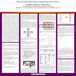
FPGA-based Modeling of Spatio-temporal Interactive Systems J. Phillips, V. Hariharan, A. Dasu, D. Peak Reconfigurable Computing Group, Utah State University jdphillips@cc.usu.edu, vignesh@cc.usu.edu, dasu@engineering.usu.edu, peakd@cc.usu.edu Processing Node Processing Node Processing Node Previous Value Divide By 2 K1 Adder Controller and Instruction Memory Processing Node Processing Node Processing Node 4-to-1 Input Mux F De- coder Divide By 2 K2 Adder N K3 Adder Processing Node Processing Node Processing Node K4 W E S Abstract Systems in the real world such as those in fluid dynamics or calcium signaling in cells or stomata networks in plants are examples of complicated real-world problems that involve a spatial organization of nodes or processing elements that interact with each other over time and influence each other over a spatial neighborhood. Attempts to model these problems using traditional software approaches generally involve extremely lengthy execution times. Field-Programmable Gate Arrays (FPGAs) naturally promote parallel processing and hold the potential to lend well to this type of spatial computing. In this research work we present an implementation of a general, application-independent FPGA-based circuit for modeling differential equation-based, spatially distributed problems. The work focuses on the specifics of the design of such a system. The internals of a single processing node are discussed, including an implementation of a Runge-Kutta fourth-order differential equation approximation algorithm. The polymorphic hardware design language Viva is introduced, and examples are given of how it is used to implement the system. The design platform of choice is a Hyper Computer from Starbridge Systems, which consists of several Xilinx Virtex II FPGAs. Details of the architecture are discussed. Techniques used to optimize the design are also discussed, including the reduction of floating-point multiplications and divisions and the tradeoff between physical circuit size and execution time. Difficulties and problems encountered are also mentioned, including issues with Viva floating-point implementations and the lack of support for double-precision floating-point numbers. Results are presented for an array of nodes that coordinate in space and time to solve simultaneous differential equations, with reference to a well observed stomata network. Comparisons between our implementation and a traditional software implementation in terms of speed and accuracy are provided, and a vision of future work is provided. Architecture #2: Generic Node with RISC Instruction Set A SIMD architecture was designed. A single controller feeds instructions to all nodes simultaneously (shown by red lines below). Each node processes its own data and stores results in its own memory. Nearest neighbor data connections are shown by the blue lines below. The controller consists of a program memory and a state machine that interprets instructions. The internals of the processing node are shown below. Four arithmetic instructions are available, as well as loads and stores. Instructions consist of 16-bit words, formatted as shown below. There are fields for the opcode, RAM address, and a select line for the input multiplexer. Figure 7 is a list of available instructions. The RAM address field can hold a number between 0 and 31, as each node has a 32 bit x 32 RAM. The select field can hold a value between 0 and 5, accessing data from one of the four neighboring nodes, an external data source, or the node’s own accumulator. Figure 8 shows a sample assembly program that has been translated into machine language by an assembler, which was created using FLEX. Design Tools and Target Platform The target hardware in this research is a single node (1 Xilinx 2V6000 FPGA) on a Starbridge Systems HC62 Hyper Computer. To facilitate interprocessor communication, the FPGA is under-clocked at 66 MHz. The design software used is Viva 2.4.2, a polymorphic, graphical hardware design language which interfaces directly with Xilinx ISE place and route tools. Node and Interconnect Basics The interconnections between processing nodes are Cellular Automata based. In other words, each processing node can communicate data with its four immediate neighbors. No concept of global data sharing exists. Each node contains hardware for performing calculations, and a private RAM that only the node in question can access. Figure 1 depicts the connections between neighboring nodes, where neighboring nodes are referred to as north, south, east, or west, respectively. Two different node architectures for solving the differential equations were proposed and tested. Details on each of the two types follows. Architecture #1: Explicit Hardware Differential Equation Solver Hardware was designed to solve the following set of equations relating to stomatal apertures in plants. The first of the two equations is a differential equation, which we solve using the 4th order Runge Kutta method, optimized for speed rather than physical circuit size. This method proved infeasible, for the following two reasons. The physical circuit size of one node consumed almost half of the Xilinx 2V6000 slices, preventing node duplication. (2) Hardware design is specific for a given equation set, meaning that the circuit must be modified if the equation set is changed. Figure 8. Assembly instructions on the left are translated into the machine code on the right. Results Final design implementation resulted in the following numbers. The controller takes 1,013 slices on the Xilinx V2P6000. Processing nodes take 3,839 slices each. It is estimated that the adder/subtractor occupies around 600 slices, the multiplier 900 slices, and around 1300 slices for the divider. Since only 1 controller node is needed, up to 9 processing nodes fit on the Xilinx 2V6000. If multiple FPGAs were available, the number of processing nodes could be increased proportionally. Figure 9 shows the speed of the algorithm coded in C running on a 1.5 GHz Intel Centrino laptop versus that of the FPGA-based SIMD computer. Notice that the FPGA-based version has the identical performance, regardless of the number of processing nodes introduced. One iteration takes about 19 microseconds. This is one of the benefits of a SIMD architecture running parallel processors. Notice also that the PC-based version requires an increasing amount of time to handle increasing nodes. This increase is linear, as expected at the rate of about 3.9 microseconds per node. From figure 9, it can be deduced that for node arrays that exceed 5 nodes, the FPGA-based implementation will yield superior results. Figure 4. SIMD Architecture. Figure 1. Node Interconnections Overview Real World NP-hard problems, such as fluid dynamics, calcium cell signaling, and stomata networks in plant leaves involve extensive computation and require unique solution methods. Field-Prgrammable Gate Arrays (FPGAs) are a potential solution to these problems, as they promote parallel processing, allow for reconfigurability, and increase processing speed. Most natural distributed systems are modeled using a set of interconnected processing nodes which solve differential equations. Each node calculates a solution to the differential equation on each time step. Data from the previous time step of other nodes is combined with a node’s own previous state to determine its current state. Runge-Kutta Approximation Algorithm The fourth-order Runge-Kutta approximation calculates the current value of a differential equation, based on the previous value, using these standard formulae: In other words, the differential function is evaluated four times to obtain each successive approximation. Figure 5. Processing Node Internals. Figure 9. Time taken by processing nodes. Captions to be set in Times or Times New Roman or equivalent, italic, between 18 and 24 points. Left aligned if it refers to a figure on its left. Caption starts right at the top edge of the picture (graph or photo). Figure 6. Instruction word format. Conclusion This research work has demonstrated the potential for FPGA use in the field of spatio-temporal interactive systems. We have shown that for a system of differential equations that model the stomatal aperture in plant leaves, a single-instruction, multiple data approach, spread across multiple arithmetic units, yields greatly superior results to that of a single processor. Future work will include recoding the node architecture in VHDL rather than Viva, since VHDL tends to create a more-efficient circuit resource-wise. The instruction set will be augmented to handle conditional branches, and instructions may be added that involve multiple arithmetic operations (e.g. multiply-and-accumulate). Figure 2. Viva example of differential function hardware Figure 7. Available Instructions. Figure 3. Dedicated hardware for Runge-Kutta solver Captions to be set in Times or Times New Roman or equivalent, italic, 18 to 24 points, to the length of the column in case a figure takes more than 2/3 of column width. Phillips Page 1 No. 161 MAPLD 2005


