Download

1 / 63
650 likes | 765 Views
Recognising Panoramas. M. Brown and D. Lowe, University of British Columbia. Introduction. Are you getting the whole picture? Compact Camera FOV = 50 x 35°. Introduction. Are you getting the whole picture? Compact Camera FOV = 50 x 35° Human FOV = 200 x 135°. Introduction.

E N D
Recognising Panoramas M. Brown and D. Lowe, University of British Columbia
Introduction • Are you getting the whole picture? • Compact Camera FOV = 50 x 35°
Introduction • Are you getting the whole picture? • Compact Camera FOV = 50 x 35° • Human FOV = 200 x 135°
Introduction • Are you getting the whole picture? • Compact Camera FOV = 50 x 35° • Human FOV = 200 x 135° • Panoramic Mosaic = 360 x 180°
Why “Recognising Panoramas”? • 1D Rotations (q) • Ordering matching images
Why “Recognising Panoramas”? • 1D Rotations (q) • Ordering matching images
Why “Recognising Panoramas”? • 1D Rotations (q) • Ordering matching images
2D Rotations (q, f) • Ordering matching images Why “Recognising Panoramas”? • 1D Rotations (q) • Ordering matching images
2D Rotations (q, f) • Ordering matching images Why “Recognising Panoramas”? • 1D Rotations (q) • Ordering matching images
2D Rotations (q, f) • Ordering matching images Why “Recognising Panoramas”? • 1D Rotations (q) • Ordering matching images
Overview • Feature Matching • Image Matching • Bundle Adjustment • Multi-band Blending • Results • Conclusions
Overview • Feature Matching • Image Matching • Bundle Adjustment • Multi-band Blending • Results • Conclusions
Overview • Feature Matching • SIFT Features • Nearest Neighbour Matching • Image Matching • Bundle Adjustment • Multi-band Blending • Results • Conclusions
Overview • Feature Matching • SIFT Features • Nearest Neighbour Matching • Image Matching • Bundle Adjustment • Multi-band Blending • Results • Conclusions
Invariant Features • Schmid & Mohr 1997, Lowe 1999, Baumberg 2000, Tuytelaars & Van Gool 2000, Mikolajczyk & Schmid 2001, Brown & Lowe 2002, Matas et. al. 2002, Schaffalitzky & Zisserman 2002
SIFT Features • Invariant Features • Establish invariant frame • Maxima/minima of scale-space DOG x, y, s • Maximum of distribution of local gradients q • Form descriptor vector • Histogram of smoothed local gradients • 128 dimensions • SIFT features are… • Geometrically invariant to similarity transforms, • some robustness to affine change • Photometrically invariant to affine changes in intensity
Overview • Feature Matching • SIFT Features • Nearest Neighbour Matching • Image Matching • Bundle Adjustment • Multi-band Blending • Results • Conclusions
Nearest Neighbour Matching • Find k-NN for each feature • k number of overlapping images (we use k = 4) • Use k-d tree • k-d tree recursively bi-partitions data at mean in the dimension of maximum variance • Approximate nearest neighbours found in O(nlogn)
Overview • Feature Matching • SIFT Features • Nearest Neighbour Matching • Image Matching • Bundle Adjustment • Multi-band Blending • Results • Conclusions
Overview • Feature Matching • Image Matching • Bundle Adjustment • Multi-band Blending • Results • Conclusions
Overview • Feature Matching • Image Matching • Bundle Adjustment • Multi-band Blending • Results • Conclusions
Overview • Feature Matching • Image Matching • RANSAC for Homography • Probabilistic model for verification • Bundle Adjustment • Multi-band Blending • Results • Conclusions
Overview • Feature Matching • Image Matching • RANSAC for Homography • Probabilistic model for verification • Bundle Adjustment • Multi-band Blending • Results • Conclusions
Overview • Feature Matching • Image Matching • RANSAC for Homography • Probabilistic model for verification • Bundle Adjustment • Multi-band Blending • Results • Conclusions
Probabilistic model for verification • Compare probability that this set of RANSAC inliers/outliers was generated by a correct/false image match • ni = #inliers, nf = #features • p1 = p(inlier | match), p0 = p(inlier | ~match) • pmin = acceptance probability • Choosing values for p1, p0 and pmin
Overview • Feature Matching • Image Matching • RANSAC for Homography • Probabilistic model for verification • Bundle Adjustment • Multi-band Blending • Results • Conclusions
Overview • Feature Matching • Image Matching • Bundle Adjustment • Multi-band Blending • Results • Conclusions
Overview • Feature Matching • Image Matching • Bundle Adjustment • Multi-band Blending • Results • Conclusions
Overview • Feature Matching • Image Matching • Bundle Adjustment • Error function • Multi-band Blending • Results • Conclusions
Overview • Feature Matching • Image Matching • Bundle Adjustment • Error function • Multi-band Blending • Results • Conclusions
Error function • Sum of squared projection errors • n = #images • I(i) = set of image matches to image i • F(i, j) = set of feature matches between images i,j • rijk = residual of kth feature match between images i,j • Robust error function
Homography for Rotation • Parameterise each camera by rotation and focal length • This gives pairwise homographies
Bundle Adjustment • New images initialised with rotation, focal length of best matching image
Bundle Adjustment • New images initialised with rotation, focal length of best matching image
Overview • Feature Matching • Image Matching • Bundle Adjustment • Error function • Multi-band Blending • Results • Conclusions
Overview • Feature Matching • Image Matching • Bundle Adjustment • Multi-band Blending • Results • Conclusions
Overview • Feature Matching • Image Matching • Bundle Adjustment • Multi-band Blending • Results • Conclusions
Multi-band Blending • Burt & Adelson 1983 • Blend frequency bands over range l
2-band Blending Low frequency (l > 2 pixels) High frequency (l < 2 pixels)