Download
1 / 78
790 likes | 945 Views
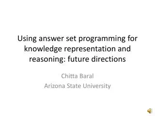
Predicate Answer Set Programming with Coinduction. Dissertation Proposal by Richard Min. Department of Computer Science The University of Texas at Dallas, Richardson, Texas, USA. 1. Introduction. Answer Set Programming (ASP)

E N D
Predicate Answer Set Programming with Coinduction Dissertation Proposal by Richard Min. Department of Computer Science The University of Texas at Dallas, Richardson, Texas, USA
1. Introduction • Answer Set Programming (ASP) • Powerful and Elegant way of a Declarative Knowledge Representation and Nonmonotonic Reasoning in Normal Logic Programming (LP). • Stable Model (Answer Set) Semantics of logic programs, by Gelfond and Lifschitz (1988) • The Term ASP due to Lifschitz, as it was recognized as a new declarative paradigm. • Implementation in the late 90’s including Smodels and Lparse by Niemelä and Simons (1996), followed by DLV, Cmodels, ASSAT, NoMoRe …
Introduction • Current implementations (of ASP solver) can handle only a class of ASP programs of “grounded version of a range-restricted function-free normal program” (Niemelä). • Grounded • Range-restricted (finite domain of constants) • Function-Free (only variables) • Normal Program (with negation allowed)
Introduction • Recent introduction of Coinductive Logic Programming (Co-LP) has been very promising to overcome many of these inherent limitations and restrictions of current ASP solvers. • Current work is an extension of our previous work for grounded (propositional) ASP solver: Gupta, G., Bansal, A., Min, R., Simon, L., Mallya, A.: Coinductive Logic Programming and Its Applications. (Tutorial Paper). In: Proc. of ICLP07, pp. 27-44. (2007).
Introduction • We achieve this novel and elegant ASP solver by co-LP with negation • Coinductive SLDNF (co-SLDNF) resolution • Co-LP with co-SLDNF provides a viable and attractive alternative to (a) current theoretical foundation and its implementation of current ASP solvers and (b) current ASP language extending to first order logic with function symbols.
1.1 Answer Set Programming • Answer Set Programming A-Prolog (Gelfond & Lifschitz), AnsProlog (Baral). According to Niemelä, • Programs are some theories (of some formal system) with a semantics assigning a collection of sets (or models, referred to as answer sets of the program) to a theory. • A program devised to solve a problem using ASP • The solutions of the problem can be derived from the answer sets of the program.
Answer Set Programming • The basic syntax of a ASP program: Lo :- L1, … , Lm, not Lm+1, …, not Ln. where Li is a literal where n 0 and n m. • Lo must be in the answer set if L1 through Lm are in the answer set and if Lm+1 through Ln are not in the answer set.
Answer Set Programming Lo :- L1, … , Lm, not Lm+1, …, not Ln. • If L0 = (or null), then its head is null (meant to be false) to force its body to be false (a constraint rule or a headless-rule), written as follows. :- L1, … , Lm, not Lm+1, …, not Ln.
Answer Set Programming • The main difficulty in the execution of answer set programs is caused by the constraint rules, including headless rules, as well as rules of the form: Lo:- not Lo, L1, … , Lm, not Lm+1, …, not Ln. Such rules are said to contain an odd-cycle in the predicate dependency graph. A program is call-consistent if it contains no odd-cycle rules. A predicate ASP program is order-consistent if none of its rules when grounded produce an odd-cycle rule (that is, well-founded and acyclic).
Answer Set Programming • Gelfond-Lifschitz Transformation (GLT) To compute the (stable) models of a program. Given a grounded program P and a candidate answer set CAS, a residual program R is obtained by applying the following transformation rules: For all literals L CAS, • To delete all rules in P which have “not L” in their body, • To delete all “L” from the bodies of the remaining rules. The least fixpoint (say, F) of the residual program R is computed by repeating this process. If F=CAS, then CAS is an answer set for P; else repeat the process with R to be CAS.
Answer Set Programming Example 1 (Gelfond-Lifschitz Transformation). Given a program P = { p :- not q. } and a candidate answer set CAS = { p }, since q is not in CAS, thus p :- not q. => p. This resulting reduct of { p } is same as CAS. Thus { p } is an answer set of P. Note that CAS can be { }, {p}, {q}, {p,q} or there is no Answer Set.
Answer Set Programming Example 2 (Gelfond-Lifschitz Transformation). Given a program P = { p :- not q. q :- not p } and a candidate answer set CAS = { p }, Since q is not in CAS, thus p :- not q. => p. q :- not p. => This resulting reduct of { p } is { p }, which is same as CAS. Thus { p } is an answer set of P.
Answer Set Programming Example 3 (GLT). Given a program P = { p :- not p. } and a candidate answer set CAS1 = { p }, since p is in CAS1, thus p :- not p. => Thus the resulting reduct of { p } is { }. Now CAS2 = { } and repeat GLT. Since p is not in CAS2, p :- not p. => p. Thus the resulting reduct of { } is { p }. Now CAS3 = { p } and repeat GLT to get CAS3 which is CAS1 and so on as CASi never converges. Thus no Answer Set.
1.2 Coinduction • Coinduction is the dual of induction. • Induction corresponds to well-founded structures that start from a basis which serves as the foundation for building more complex structures.
Induction and Coinduction • Induction is a mathematical technique for finitely reasoning about an infinite number of things. • If there were only finitely many different things, than induction would not be needed. • Naturals: 0, 1, 2, … • The naïve “proof” • 3 components of inductive definition: (1) Initiality, (2) iteration, (3) minimality • for example, a list is defined inductively (1) [ ] – an empty list is a list (initiality) (2) [ H | T ] – a list if T is a list and H is a list (iteration) (3) nothing else is a list (minimality)
Induction and Coinduction • Coinduction is a mathematical technique for finitely reasoning about infinite things. • Mathematical dual of induction • If all things were finite, then coinduction would not be needed. • Perpetual programs, • Infinite strings: networks, model checking • 2 components of coinductive definition: (1) iteration, (2) maximality • For example, a list is defined coinductively (1) [ H | T ] is a list if T is a list and H is a list (iteration). (2) The set of lists is the maximal set of such lists.
Mathematical Foundations • Duality provides a source of new mathematical tools that reflect the sophistication of tried and true techniques.
Example: Natural Numbers • (S) = { 0 } { succ(x) | x S } • N = • where is least fixed-point. • aka “inductive definition” • Let N be the smallest set such that • 0 N • x N implies x + 1 N • Induction corresponds to LFP interpretation.
Example: Natural Numbers and Infinity • (S) = { 0 } { succ(x) | x S } • unambiguously defines another set • N’ = = N { } • = succ( succ( succ( ... ) ) ) = succ( ) = + 1 • where is a greatest fixed-point • Coinduction corresponds to GFP interpretation.
Applications of Coinduction • model checking • bisimilarity proofs for process algebras • lazy evaluation • reasoning with infinite structures • perpetual processes • cyclic structures • operational semantics of “coinductive logic programming”
Infinite Objects and Properties • Traditional logic programming is unable to reason about infinite objects and/or properties. • Computer Network example: perpetual binary streams (as traditional logic programming cannot handle). • For example, bit-stream of a bit-pattern bit(0). bit(1). bitstream( [ H | T ] ) :- bit( H ), bitstream( T ). |?- X = [ 0, 1, 1, 0 | X ], bitstream( X ).
Rational Tree and Proof Let node(A, L) be a constructor of a tree with root A and subtrees L, where A is an atom and L is a list of trees. • A tree is rational if the cardinality of the set of all its subtrees is finite. An object such as a term, an atom, or a (proof or derivation) tree is said to be rational if it is modeled (or expressed) as a rational tree. (2) A rational proof of a rational tree is its rational solved form computed by rational solved form algorithm. (3) A coinductive proof of a rational (derivation) tree of program P is a rational solved form (tree-solution) of the rational (derivation) tree.
Coinductive Hypothesis Rule • Coinductive hypothesis rule: (Simon et al. 2006) states that during execution, • If the current resolvent contains a call C’ that unifies with an ancestor call C encountered earlier, then the call C’ succeeds; the new resolvent is R’ where = mgu(C, C’) and R’ is obtained by deleting C’ from R. Ex. Program with C1: { p(X) :- p(f(X)). }, Query ?- p(X). { p(X) } [C1 head] {p(f(X)) } [C1 body, =mgu(p(X), p(f(X))) => X=f(X)] { }.
Coinductive Hypothesis Rule • With this rational feature, co-LP allows programmers to manipulate rational (finite and rationally infinite) structures in a decidable manner. • To achieve this feature of the rationality, the unification has to be necessarily extended, to have “occur-check” removed. • Unification equations such as X=[1|X] are allowed in co-LP (that is, an infinite sequence or stream of 1, or a rational tree consisting of two nodes where the root node points to a node of 1 and to itself). • In fact, such equations will be used to represent infinite (regular) structures in a finite manner.
Co-SLD Resolution • Co-SLD Resolution is very similar to SLD Resolution. Thus, given a call during execution of a logic program, the candidate clauses are tried one by one via backtracking. • Under co-SLD resolution, apply the coinductive hypothesis rule to check if the current call will unify with any of the earlier calls. • If there is a cycle (or a circle) in the path of the execution, it will be detected by co-SLD and infinite traversal of this cycle stopped.
2. Thesis Proposal • Design of “Coinductive Logic Programming” language extended with negation as failure (co-LP with co-SLDNF resolution). • Designing a simple and efficient implementation technique to implement co-LP with co-SLDNF atop an existing Prolog engine. • Proof of the correctness (soundness and completeness) of co-SLDNF resolution.
Thesis Proposal 4. Design of a Top-Down algorithm for goal-directed execution of propositional and predicate Answer-Set Programs. 5. Design of a simple and efficient implementation technique to implement the Top-Down propositional and predicate ASP atop an existing Prolog engine. 6. Prototype implementation of co-ASP Solver
3. Co-LP with Negation • Co-LP with co-SLD was initially designed only for definite logic programs (that is, without negation). • Thus the extension of co-LP to provide negation (that is, to have a negative literal) is somewhat natural and inevitable for research endeavor to extend the scope of co-LP to infer negative information and reason with negation.
Co-LP with Negation • Negation causes many problems in logic programming (e.g., nonmonotonicity). • For example, one can write programs whose meaning is hard to interpret (e.g., p :- not p. ) whose completion is inconsistent or execution is infinite). • However, there are many benefits and advantages to have negation in logic programming so that one may represent, reason and infer “what is not” in a Database or a Knowledgebase.
Co-LP with Negation • Two major inference rules dealing with negation are: • the closed world assumption (CWA) introduced by Reiter, and (2) the negation as failure introduced by Clark. • We choose negation as failure for co-LP, to be consistent with the semantics of SLDNF of the underlying Prolog engine. • We term the operational semantics of co-LP extended with negation as failure coinductive SLDNF resolution (co-SLDNF resolution).
Co-SLDNF Resolution • Extending co‑SLD to co‑SLDNF, • the goal ?- nt(A). succeeds (or has a successful derivation) if A fails; • likewise, the goal ?- nt(A). fails (or has a failure derivation) if the goal ?- A. succeeds. • In co‑SLDNF (contrast to SLDNF), • any successful negated goals will be remembered as any negated goals can also succeed coinductively.
Co-SLDNF resolution • Co-SLDNF resolution extends co-SLD resolution with negation. • Essentially, it augments co-SLD with the negative coinductive hypothesis rule, stating: If a negated call not(p) is encountered during resolution, and another call to not(p) has been seen before in the same computation, then not(p) coinductively succeeds.
Co-SLDNF resolution • To implement co-SLDNF, • the set of positive and negative calls has to be maintained in • positive hypothesis table (denoted +) and • negative hypothesis table (denoted -) respectively. • Note that nt(A) below denotes coinductive “not” of A. • Note that denotes an empty clause { }.
Co-SLDNF resolution Definition (Co‑SLDNF Resolution): Suppose we are in the state (G, E, +, -) where G is a list of goals and E is a set of substitutions (environment). + is Positive Hypothesis Table, and - is Negative Hypothesis Table. Consider a subgoal A G: .
Co-SLDNF resolution: (+,+), (-,-) (1) If A occurs in positive context (i.e., under even number of negations), and A’ + such that = mgu(A,A’), then the next state is (G’, E, +, -), where G’ is obtained by replacing A with . • If A occurs in negative context (i.e., under odd number of negations), and A’ - such that = mgu(A,A’), then the next state is (G’, E, +, -), where G’ is obtained by A with false.
Co-SLDNF resolution: (+,-), (-,+) (3) If A occurs in positive context, and A’ - such that = mgu(A,A’), then the next state is (G’, E, +, -), where G’ is obtained by replacing A with false. (4) If A occurs in negative context, and A’ + such that = mgu(A,A’), then the next state is (G’, E, +, -), where G’ is obtained by replacing A with .
Co-SLDNF resolution: Expansion (5) If A occurs in positive context, then the next state is (G’, E’, {A} +, -), where G’ is obtained by expanding A in G via normal call expansion with E’ as the new system of equations obtained. (6) If A occurs in negative context, then the next state is the (S1 or … or Sn) where Si is (G’i, E, +, {A}-) for each clause Ci (where 1≤ i ≤ n) whose head atom is unifiable with A. Thus each G’i is obtained by expanding A in G via normal call expansion with Ci. Note that we require A to be ground, and therefore E is unchanged.
Co-SLDNF: negation as failure (7) If A occurs in positive or negative context and there are no matching clauses for A, and there is no A’ (+ -) such that A and A’ are unifiable, then the next state is (G’, E, +, {A} -), where G’ is obtained by replacing A with false. (8) (a) nt(…, false, …) reduces to , and (b) nt(A, , B) reduces to nt(A, B) where A and B represent conjunction of subgoals.
Co-SLDNF resolution Note (i) step (5) and (6) may be non-deterministic (ii) the result of expanding a subgoal with a unit clause in step (5) and (6) is an empty clause (), (iii) when an initial query goal reduces to an empty clause (), it denotes a success, (iv) that “or” in step (6) is defined as follows: • (Si or (, E, +, -)) = ((, E, +, -) or Si) = (, E, +, -), • (Si or (false, E, +, -)) = ((false, E, +, -) or Si) = Si, and • ((false, E, +, -) or (false, E’, +’, -’)) = (false, E, +, -).
Co-SLDNF derivation Co-SLDNF derivation of the goal G of program P is a sequence of co-SLDNF resolution steps with a selected subgoal A, consisting of (1) a sequence (Gi, Ei, χi+, χi-) of state (i 0), of (a) a sequence G0, G1, ... of goal, (b) a sequence E0, E1, ... of mgu's (substitutions), (c) a sequence χ0+, χ1+, ... of the positive hypothesis tables, (d) a sequence χ0-, χ1-, ... of the negative hypothesis tables, where (G0, E0, χ0+, χ0-) = (G, , , ) is the initial state, and
Co-SLDNF derivation (2) for Definition (co-SLDNF resolution) (5-6), a sequence C1, C2, ... of variants of program clauses of P where Gi+1 is derived from Gi and Ci+1 using θi+1 where Ei+1 = Eiθi+1 and (χi+1+, χi+1-) as its resulting positive and negative hypothesis tables. (3) If a co‑SLDNF derivation from G results in an empty clause of query , that is, the final state of (, Ei, χi+, χi-), then it is a successful co‑SLDNF derivation, and a derivation fails if a state is reached in the subgoal-list which is non-empty and no transitions are possible from this state.
Co-SLDNF derivation C1,θ1 (G0, E0, χ0+, χ0-) C2,θ2 (G1, E1, χ1+, χ1-) C3,θ3 (G2, E2, χ2+, χ2-) ... And a successful co-SLDNF derivation will result in: ({ }, En, χn+, χn-).
Example - NP1 Consider the following program (NP1): NP1: p :- nt(q). q :- nt(p). The query ?- nt(p) will generate the following transition sequence: ({ nt(p) }, { }, { }, { }) by (6) ({ nt(nt(q)) }, { }, { }, {p}) by (5) ({ nt(nt(nt(p))) }, { }, {q}, {p}) by (2) • ({ }, { }, {q}, {p}) [success]
Example – NP1 • Note that the query ?- p will also succeed (p nt(q) nt(nt(p)) success) • NP1 has two fixed points namely {p} and {q}. • The query ?- nt(p) is true in {q}, while the query ?- p is true in {p}. Thus, computing with greatest fix point semantics in presence of negation is always troublesome, since one has to be careful that given a query, different parts of the query are not computed w.r.t. different fixed points. • Thus, the query ?-p, nt(p) will never succeed if we are aware of the context (of a particular fixed point being used).
Example - -Automata • The -Automata consists of 4 states of {s0, s1, s2, s3} and 5 events of {bootup, work, crash/off, shutdown, booterror, reboot}. • This example models the operation of a computer. The corresponding co-LP program code that models the automata is as follows:
Example - -Automata state(s0,[s0|T]):-event(bootup), state(s1,T). state(s1,[s1|T]):-event(work), state(s1,T). state(s1,[s1|T]):-event(crash/off), state(s2,T). state(s2,[s2|T]):-event(shutdown), state(s0,T). state(s0,[s0|T]):-event(booterror), state(s3,T). state(s3,[s3|T]):-event(reboot), state(s0,T). event(bootup). event(work). event(crash/off). event(shutdown). event(booterror). event(reboot).
Example - -Automata The query ?- state(S,T) may generate all possible paths, each ending with a cycle whereas the query ?- state(X,T), X=s0 will narrow the results to cycles starting from state s0 (** denotes a (rational) infinite list). 1 X = s0, T = [s0, s1|**] ; 2 X = s0, T = [s0, s1, s2|**] ; 3 X = s0, T = [s0, s3|**]
Example - -Automata The query ?- state(X,T), nt(state(s0,T)). shows cycles that do not start with s0. 1 X = s1, T = [s1|**] ; 2 X = s1, T = [s1, s2, s0|**] ; 3 X = s1, T = [s1, s2, s0, s3|**] ; 4 X = s2, T = [s2, s0, s1|**] ; 5 X = s2, T = [s2, s0, s1|**] ; 6 X = s2, T = [s2, s0, s3|**] ; 7 X = s3, T = [s3, s0, s1|**] ; 8 X = s3, T = [s3, s0, s1, s2|**] ; 9 X = s3, T = [s3, s0|**]
Declarative Semantics of co-SLDNF • The declarative semantics of co-SLDNF is based on the work of Fitting (Kripke-Kleene semantics with 3-valued logic, extended by Fages for stable model with completion of program). • The detailed account of co-SLDNF can be found in our Technical Report.