Download
1 / 25
250 likes | 344 Views
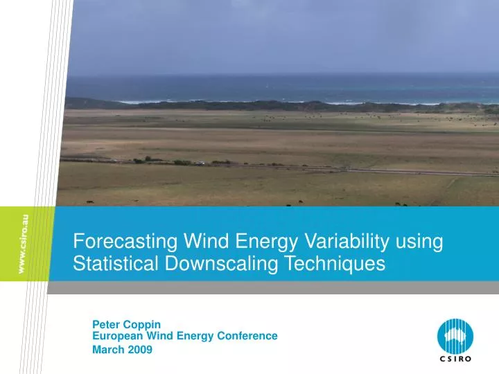
Peter Coppin European Wind Energy Conference March 2009. Forecasting Wind Energy Variability using Statistical Downscaling Techniques. Acknowledgements. Division of Marine and Atmospheric Research Robert Davy (principal researcher) Milton Woods Chris Russell Peter Coppin

E N D
Peter CoppinEuropean Wind Energy Conference March 2009 Forecasting Wind Energy Variability using Statistical Downscaling Techniques
CSIRO. Forecasting Wind Energy Variability Acknowledgements Division of Marine and Atmospheric Research • Robert Davy (principal researcher) • Milton Woods • Chris Russell • Peter Coppin Funded by the Australian Government – Department of Resources Energy and Tourism (DRET) • Australia Wind Energy Forecasting System (supplied by ANEMOS) In collaboration with • Australian Bureau of Meteorology • European Union Framework 7 “SAFEWIND” Project partners
CSIRO. Forecasting Wind Energy Variability Core wind generating area SE states 35,000MW max demand
CSIRO. Forecasting Wind Energy Variability Typical winter / early spring conditions
CSIRO. Forecasting Wind Energy Variability IR Satellite image – 1225 hr on Sept 11 2004 showing organised convection
CSIRO. Forecasting Wind Energy Variability Example of problem – high variability in South Australia High wind variability at moderate wind speeds large swings in aggregate wind power wind farm aggregation can amplify the absolute magnitude of power changes variation can exceed available spinning reserve response capability State total generation Generation in 6 regions Regional Generation at 12:30
CSIRO. Forecasting Wind Energy Variability Steps to forecasting wind variability • Create a numerical index to describe severity • Calculate index for observations • Formally correlate observed variability with weather patterns derived from Numerical Weather Prediction (NWP) products via EOF analysis • Produce prediction of variability based on combination of important patterns – using Random forest techniques – express in terms of wind speed and wind energy production ramp rate at suitable forecast time horizon • Check predictability with observations (separate data segment)
CSIRO. Forecasting Wind Energy Variability Modelling wind variability Initial proof-of principle based on analysis fields (i.e. not forecast mode) • NCEP Global Tropospheric Analyses ( ds083.2 ) • six hourly meteorological fields at 1.0° resolution [1999 - ] • Surface wind speed measurements: • 6 locations across South eastern Australia • Used for calculating variability index and validation Forecast mode trial • Bureau of Meteorology W-LAPS model • Six hourly fields at 1° and 0.1° grids (data set length?) • 12 hours ahead
CSIRO. Forecasting Wind Energy Variability Index of wind variability from Woods, Davy & Coppin, 2007 Variability index is six hour running standard deviation of 2 hour high-pass filtered (10min) raw data
CSIRO. Forecasting Wind Energy Variability Available (and relevant) variables for EOF analysis NCEP Global Tropospheric Analyses ( ds083.2 ) six hourly meteorological fields at 1.0° resolution [1999 - ] Geopotential height Air temperature Relative humidity U wind speed V wind speed Vertical velocity Absolute vorticity Height of planetary boundary layer Precipitable water Cloud water Lifting index Convective inhibition Convective available potential energy etc
CSIRO. Developing a prediction of wind variability EOF example : Temperature
CSIRO. Forecasting Wind Energy Variability Quantitative modelling Empirical model(random forest) Sum of variability indexat 6 sites Meteorological inputs(transformed using EOF) Model period: 2003-4
CSIRO. Forecasting Wind Energy Variability Winter – important patterns explaining variability Height of planetary boundary layer – EOF1 Absolute vorticity – EOF3 Velocity component V – EOF2
CSIRO. Forecasting Wind Energy Variability NCEP Results – winter / early spring • Prediction of variability index (using analysis NWP products) Aggregate 6 locations in SE Australia Important predictors: EOF number Height of planetary boundary layer 1 Absolute vorticity 3 V wind speed 2 U wind speed 1 R2=0.74
CSIRO. Forecasting Wind Energy Variability NCEP Results – winter / early spring • Prediction of variability index (using analysis NWP products) Aggregate 6 locations in SE Australia Single site Important predictors: EOF number Height of planetary boundary layer 1 Absolute vorticity 3 V wind speed 2 U wind speed 1 R2=0.74
CSIRO. Forecasting Wind Energy Variability Summer – important patterns explaining variability Cloud water – EOF1 Convective available potential energy – EOF1 Geopotential height – EOF2
CSIRO. Forecasting Wind Energy Variability NCEP Results - summer Prediction of variability index (using analysis NWP products) Aggregate 6 locations in SE Australia Important predictors: EOF number Cloud water 1 Geopotential height 2 CAPE 1 V wind speed 2 R2=0.66
CSIRO. Forecasting Wind Energy Variability NCEP Results - summer • Prediction of variability index (using analysis NWP products) Aggregate 6 locations in SE Australia Single site Important predictors: EOF number Cloud water 1 Geopotential height 2 CAPE 1 V wind speed 2 R2=0.66
CSIRO. Developing a prediction of wind variability Mean wind power ramp rate modelling Modelling of 6-hour mean ramp rate • aggregate power from 6 locations vs fitted variability index
CSIRO. Forecasting Wind Energy Variability Short-term wind power ramp rate modelling • Modelling of 10 min ramp rate • aggregate power from 6 locations (normalised) • relationship of 6 hourly maximum ramp rate (left) and instantaneous ramp rate (right) to variability index
W-LAPS forecast mode trial • EOF analysis uses both 1° (100km) and 0.1° (10km) fields • Correlations performed on 12-hour ahead forecast products • Single site results available • Example EOF model fit: CSIRO. Forecasting Wind Energy Variability
CSIRO. Forecasting Wind Energy Variability W-LAPS Results – 12 hours ahead • Forecast of variability index (using analysis NWP products) • Single site Winter Summer
CSIRO. Forecasting Wind Energy Variability W-LAPS Results – 12 hours ahead • Forecast of variability index (using analysis NWP products) • Aggregate of several sites in one state Winter Summer
CSIRO. Forecasting Wind Energy Variability Further work Implement working system ready for coding into ANEMOS system as a module Further validate forecast-mode models for aggregate variability requires additional surface data Quantify value to system operators of variability information cost benefit analysis
Thank you Contact Us Phone: 1300 363 400 or +61 3 9545 2176 Email: enquiries@csiro.au Web: www.csiro.au Centre for Australian Weather and Climate Research A partnership between CSIRO and the Bureau of Meteorology Robert Davy Phone: 02 6246 5604 Email: robert.davy@csiro.au Web: www.csiro.au/weru